Now that the 2019-2020 season has ended, let’s take a quick look at something almost every data scientist knows: polynomial projection. Now, if you’re a data scientist and find yourself mumbling, “I’ve never heard of that,” don’t worry: You have.

Over the next few posts, we are going to discuss a larger problem of approximating polynomial curves and their role in particular player capabilities, ultimately leading to an analysis of actions on the court and the associated decision making process that folks really like to discuss but rarely quantify; at least in a public setting.

To start, we look at the mechanical process of fitting a polynomial. What we mean by mechanical is purely the art of fitting a curve to data, not the scientific process. To this respect, we eschew the required exploratory data analysis required to for fitting a model to a collection of observations. The goal at this point is to simply fit a curve using a mathematical model, with utter disregard of the statistical properties. Why do it this way? Simple, this is the baseline for how neural networks and support vector machines work.

So let’s begin with a simple, yet excessively controversial topic: Career Arcs and “proof” of the Greatest of All-Time*.

Career Arcs

It is commonly accepted that a player’s career moves in an arc. Players are introduced into the league and must assimilate to find their own value added, creating a gradual increase in value before hitting a ‘peak’ potential and gradually decreasing as father time begins to get the better of their bodies.

At this point, discussion of “value” becomes the prime topic of conversation and if you take a glimpse, you can find several articles dedicated to one number metrics such as RAPM, RPM, RAPTOR, BPM, and PIPM, to name a few. Several pro teams have their own “in-house” plus-minus all-in-one metrics, which include models I’ve seen called “Robust Plus-Minus,” “Win-Probability Plus-Minus,” and “Tracking Plus-Minus.” Each method attempts to take specific components of the game and quantify each set of actions into a ‘value added’ by that player. A target for such a model’s success is to adequately predict over 60% of ratings for particular stints. Most metrics tend to dance about 63-65% out-of-sample prediction error; while the best in-house metric I have seen routinely hit 70%. Despite the 70%, there are still issues with that model.

Of all public metrics, the one I have come to trust the most over the past few years has been PIPM. This is not an endorsement to suggest PIPM is the correct choice, but rather one that doesn’t have as wide-spread variability such as RAPM and therefore the one I will use for the purpose of this study: show the mechanical process of generating a career arc.

Let’s start with an example.

Charles Barkley: 1985 – 2000

Charles Barkley, drafted fifth by the Philadelphia 76ers in 1984, played for a total of three teams over a sixteen season career. Considered one of the greatest forwards in history, a member of the NBA Hall of Fame, Chuck provided immense value to his teams, including a run at the 1993 NBA Finals with the Phoenix suns as the league’s Most Valuable Player. Using PIPM, we can yield a quantification of his value:

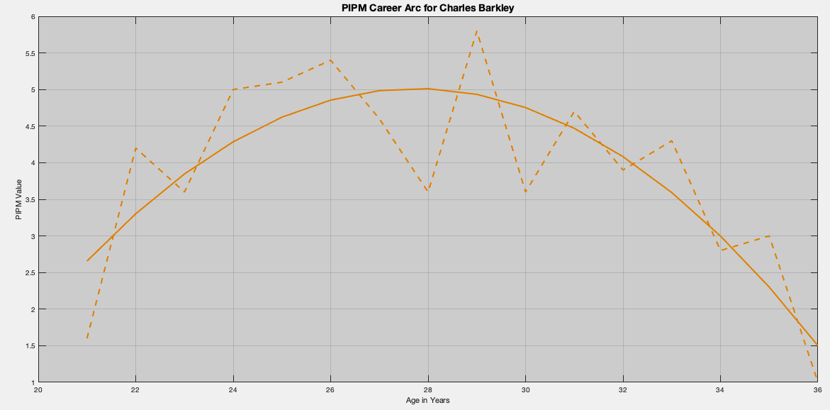
Here, we immediately see the mechanical solution of the career arc for Charles Barkley. Despite PIPM looking fairly noisy, the smoothed arc looks like a really good fit. It captures everything we expect in a player’s career arc:

• Gradual build up to a peak.
• Peak at roughly about the age of 28 years.
• Gradual decrease until retirement.

So how do we go about fitting this polynomial to the PIPM estimates?

Step 1: Determine an Appropriate Model**

Our first step is to determine an appropriate model. The goal of creating a model is to define a set of parameters that succinctly contains the information content of the data, but in a meaningful way to accurately portray future observations while illustrating past observations. To this effect, the most common polynomial projection model is linear regression.

The linear regression model projects data onto a linear set of parameters, called coefficients. This can be confusing to novices because models such as

is a linear model, despite the squaring and exponential function! This is because the coefficients are linear. For those familiar with the R and Python packages of ridge regression, Poisson regression, logistic regression, or even multi-layer neural networks with even soft-max or sigmoid functions, guess what… they are all linear models.

For our model, we naively follow the trail of ‘player improves to peak and then gradually declines.” To this end, we build a quadratic polynomial, defined by

Since we impose a quadratic model, we should expect all career arcs to be concave down. That is, all polynomials point downward. This will always guarantee an apex for a player’s career arc.

In another decision, we use a player’s age in years as the dependent variable. This is making the assumption that players will typically play, at baseline, in the same ages and that bodies are growing and declining at approximately the same rate. This also helps avoid the question of “but what about this 28 year old rookie?” we typically get when using years of experience as the factor.

Parameter Interpretation

Now given the model, we have three parameters of interest: Beta Zero, Beta One, and Beta Two. Beta Zero is the ‘height’ adjuster of the career arc. Its literal interpretation in this context is the ‘value of PIPM when a player is born.” However, there are no babies in the NBA; no matter how much you claim your most hated player is such. Therefore, we look at the real interpretation here: Beta Zero adjusts the high of the career arc. that is, if we subtract Beta Zero, the shape of the polynomial stays exactly the same, but the polynomial moves up or down, depending on the directionality of Beta Zero.

Beta Two identifies the sharpness of a players increase and decrease in value. This value must be negative is order to generate a career arc. This is the value that determines if a quadratic points downward. If this value is close to zero, the career arc will be slowly moving. If the magnitude of Beta Two is large, the career is most likely very short.

Finally, Beta One is the “peak-finder” of the career arc; or rather left-right movement. The affect of this term is best seen in completing the square by putting the polynomial into “h-k” form:

Recall that Beta Two must be negative. This suggests that Beta One must be non-negative, otherwise the career arc will be in negative years. In fact, from this form, we will see that a player’s peak is estimated to be

which must be a positive value, as no players yield maximum PIPM values prior to birth.

Step 2: Solve the Regression

Once we have determined the model, next we must perform the actual mechanical process of determining the coefficients. The reason we keep saying “mechanical” is because, again, we are eschewing statistical reasoning. We have not looked at the distributions of PIPM over age, performed a study on the effects of age on PIPM; nor have we performed a qualitative study on the captured effects of the game on PIPM, conditioned on player type, scheme, strength of stint, condition of game, etc. Instead, we are applying a mathematical technique to data and saying “viola!”

To do this, we write the model in terms of a system of algebraic equations and solve using a standard technique that every data scientist knows: least squares.

In case you are unfamiliar with least squares, let’s apply this to Charles Barkley’s PIPM values. Sir Charles started playing at age 21 and completed his career at age 36. Therefore, our “X” values will be 21 through 36. Since we are using a constant coefficient, Beta Zero, and a square coefficient, Beta Two, we should also have constant years and squared years! Therefore, we have the system of equations

where PIPM values are identified from Jacob Goldstein’s site, Wins Added. Least squares puts these equations into a matrix form and then “solves” the equation by minimizing least-square error.

That is, the above equations are written in matrix form as:

This is commonly written as Y = XB form. The obtain the least-squares solution, we solve for the minimum of square error loss:

Solving this is an exercise in differentiability:

Solving this last equation for zero is the least-squares solution. Taking yet another derivative will prove that it is indeed a minimum. Applying this to Charles Barkley’s data, we apply the MATLAB code:

This gives us Beta Two as -0.0517, which is indeed negative! This also yields the career peak at 27.7545 years. This again is exactly what we expect.

Implicit Decisions!

Note that the process of thinking through a model that makes sense, and using a mathematical technique that has been taught for centuries, we still made an implicit statistical assumption about our data. Explicitly, the use of a square-error loss function is equivalent to the assumption of homoscedastic (constant variance) Gaussian noise on the data; as the Euclidean loss function is the negative-log-likelihood of the Gaussian model!

Therefore, if we are to make any further descriptions of the model, we should perform the required exploratory data analysis to ensure that this implicit Gaussian noise assumption is indeed a correct one to make.

Again, overtly eschewing this requirement for the sake of seeing how we obtain a smoother that descriptively illustrates a player’s career arc, we proceed by looking at various over players. Such as…

Larry Bird: 1980 – 1992

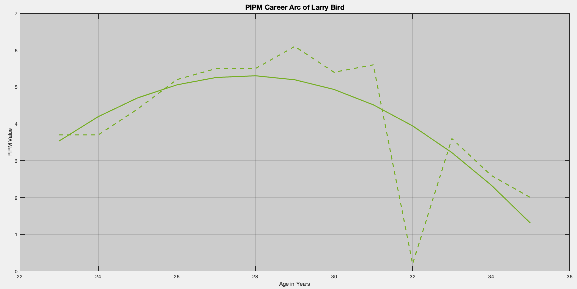
Larry Bird’s coefficients are a little sharper than Barkley’s suggesting a stronger decline; which coincides with his back injuries later in his career. With a coefficient set of -54.2795, 4.2874, -0.0771; we find that Bird’s peak year was at age 27.7960; which is the 1984-85 NBA season, the middle of his three consecutive MVP awards!

Magic Johnson: 1980 – 1991, 1996

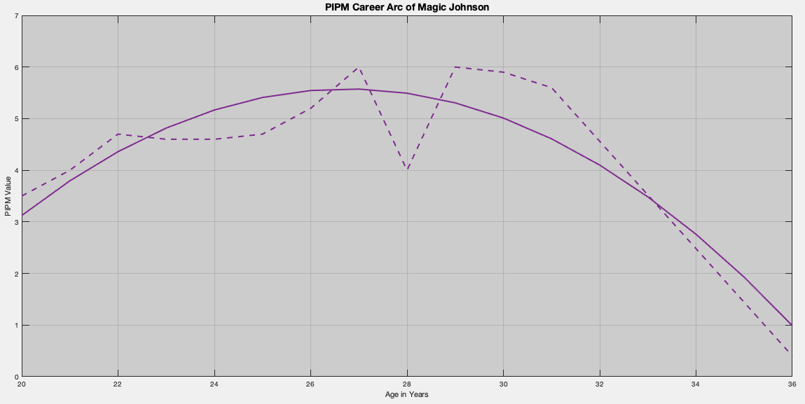
Magic Johnson, similar to Larry Bird, dominated the 1980’s and suffered health disruptions early into the 1990’s. Unlike Bird, Magic attempted a slight comeback late in his career during the 1995-96 (1996) NBA season. Since we are applying a simple regression model, and have “enough” data, we can capture the “predicted” PIPM values for the years missed. Granted, these predictions must be taken with a grain of salt as we did not perform the necessary analysis to validate the model.

That said, Magic’s coefficient set is -32.8756, 2.8740, -0.0537; which indicates a decline much like Charles’ Barkley’s. This is identified through the -0.05 value. Different from Barkley, is Magic’s -32, which is a couple points better than Barkley’s. This indicated Magic had a “better” career than Barkley’s.

It should be noted that, due to his harsh decline after five years off, the mechanical process becomes biased towards his younger years, making for a peak age of being 26.7578 years, which was the 1986-87 NBA season.

The ability to identify missing years allow us to look at one very particular player…

Michael Jordan: 1985-1993,1995-1998,2002-2003

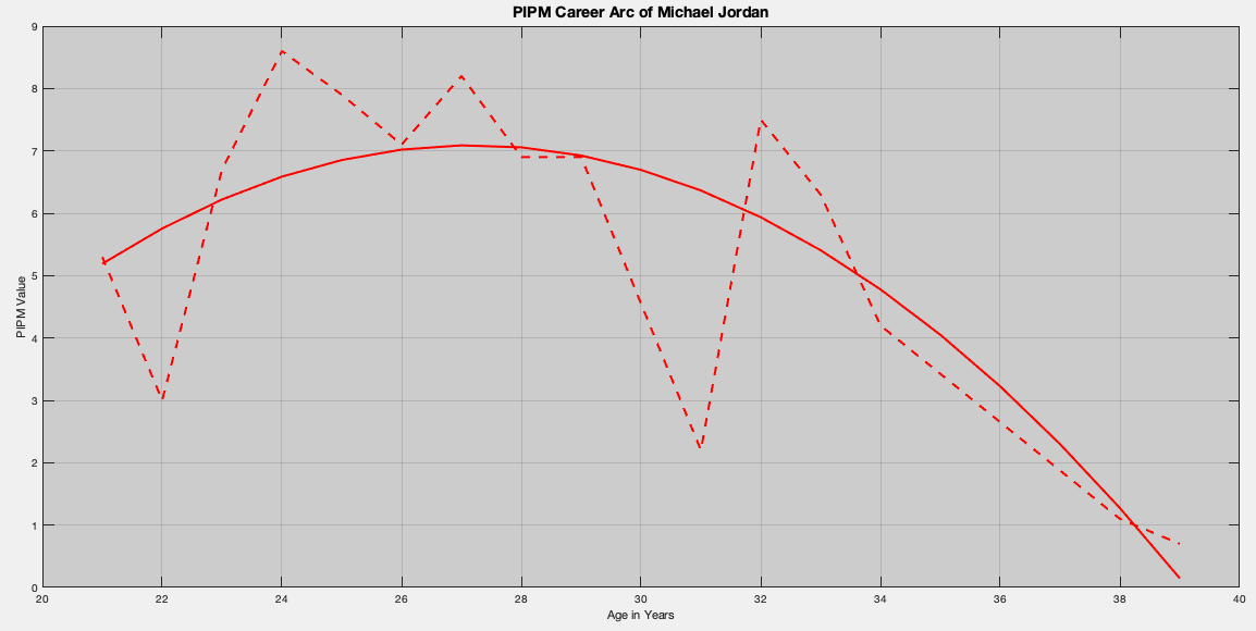
Michael Jordan, with two missing stints within his career, can be identified using the mechanical process. The graph looks like a rapid decline, but don’t let the visual fool you. Jordan’s coefficients are -29.6335, 2.7021, -0.0497. This indicates of the four players so far, Jordan has the slowest decline and the highest height setter. That is, Jordan is viewed as the GOAT of this pack of four players.

Here, Jordan’s peak is listed at 27.1813 years, which is the 1991 NBA season; the beginning of his dynastic run after thwarting the Detroit Pistons.

Selected Players

Let’s start combining many players of interest. Here, we include not only the four players above, but also some other notable players from the 1973-present era: Kareem Abdul-Jabbar, Julius Erving, Shaquille O’Neal, Kobe Bryant, and even Dominique Wilkins; as he is viewed as a superstar but never quite a perennial MVP caliber player.

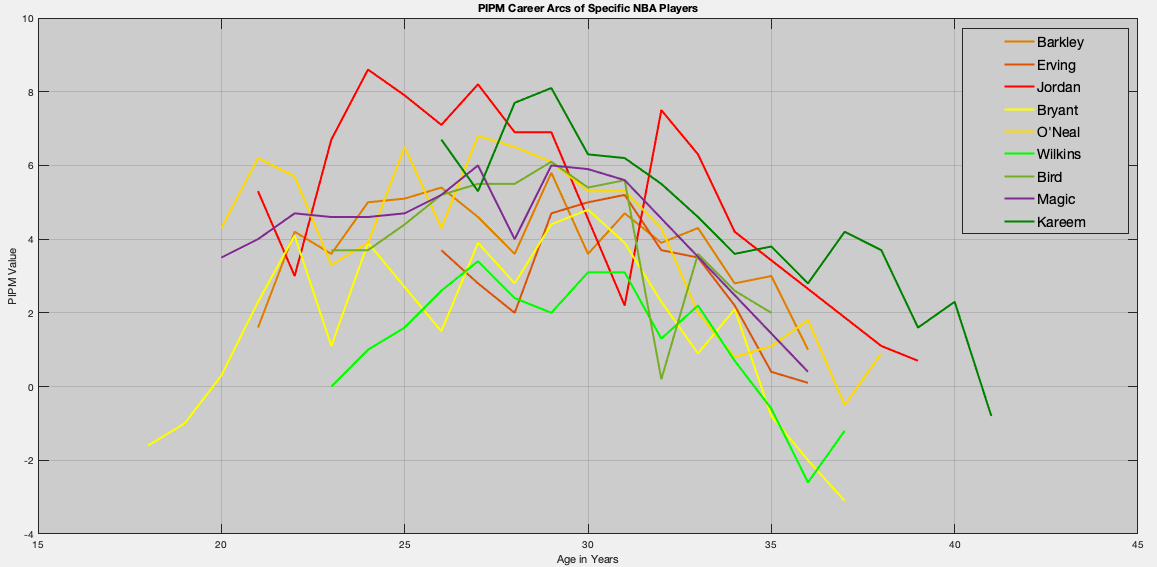
This graph looks like a mess! Let’s apply a mechanical polynomial projection algorithm; in this case quadratic polynomial regression, to obtain a “cleaner look.”

Here we see dominated convergence of two players: Michael Jordan and Kareem Abdul-Jabbar. That is, every other PIPM line is completely below theirs. Of course, Jordan and Kareem intersect at different years. This is an illustration of the maximum greatness versus sustained greatness argument.

As expected, we see a great player like Dominique note quite reach the level of the other Hall of Fame players. But more importantly, we see the career arc of Charles Barkley follow very closely to Larry Bird’s career arc. In effect, this illustrates that Barkley was indeed a championship level player, but had many factors against him: luck of the draw (match-ups), allied fire-power (sorry Cliff Robinson and Mike Gminski, you’re no match for Robert Parish, Kevin McHale, and Dennis Johnson), and competitive star-power (damn you Michael Jordan, Hakeem Olajuwon, and Stockton/Malone!).

But let’s make this a little more interesting…

Here Comes LeBron…

Since LeBron James has already played an entire Hall-of-Fame career, we can apply this same methodology and compare his career arc to PIPM data. In doing so, we observe LeBron’s coefficient set to be -46.5947, 3.8412, -0.0680.

This suggest LeBron is much more like Michael Jordan’s apex with durability like Charles Barkley. In fact, it can be argued that James’ apex is better than Jordan’s, but with less longevity than Jordan’s! Strange to suggest, as LeBron has played longer than Jordan, but yet Jordan had “better” early years and James’ final years (primarily age 39) have yet to play out.

Which brings us to the important point of this post…

DO NOT USE MECHANICAL PROCESSES TO FORECAST!

Despite the out-of sample errors being viewed as “good,” these methods are considerably poor at forecasting when it matters the most: selecting monetary value of a player, predicting wear and tear of the body, and understanding impact within scheme. The reason the above looks so pretty is that every one of the above players were great.

If we were to apply this methodology to say, Isaiah Thomas, we will be greatly disappointed in the results. Instead, a more robust methodology must be selected. Either by parametric methods that rely on the stochasticity of a player, or by nonparametric methods that learn on similar players that have played before them, such as a random forest.

To reiterate, the goal of this post is to show smoothing and introduce a familiar and easy concept to see smoothing in action. In our follow-up post, we will look at a stochastic model for a different process that uses quadratic regression.

But for now, let’s continue the debate of who is the GOAT. 🙂

*GOAT is only relative to PIPM and what PIPM measures. Not actual, definitive proof of being the GOAT.

**We call this a “appropriate model” only because it’s a mathematical model. We have not proven this is an “appropriate” statistics model by any means.