With the highest return for a field goal attempt per possession being a three point field goal, teams have caught on that three point field goals are the optimal way to go on offense provided they have consistently accurate shooters from that range. This qualifier has been the difficult part of the three point equation. Some teams, such as Grinnell College devised game plans to increase the number of three point field goal attempts per possession while most teams looked for shooters with high three point field goal range. In the late 80’s / early 90’s these players were quite rare. During these years, top 10 shooters would convert roughly 55% percent of their attempts; premier players topping 60% such as Charles Barkley (.632 in 1990, .614 in 1991).
This means that if a team wanted a “Charles Barkley” type scorer from beyond the arc, they would have to pony up at .421 3PFG%. To be an equivalent top 10 shooter from beyond the arc, a team would look for shooters with .367% from beyond the arc. In these cases, the shooters would be equivalent to their counterparts. There were indeed 18 such players who somewhat fit the bill. They had at least one attempt per game played, shot better than 36.7% from beyond the arc, and played at least half the season. But only eleven of these players attempted 2 or more attempts per game. Meanwhile, David Robinson was taking 16.6 two point field goal attempts per game and converting 55.4% of these attempts. This meant that the shooters were not negating the effects of top ten scorers. In truth, these shooters would require 11 attempts per game consistently just to nullify the top ten scorers of this era. The only player to get above 4 attempts per game in the 1991 season? Dennis Scott with 4.1 attempts. Compare this today to Stephen Curry, who has averaged 11.2 and 10.0 attempts per game in the 2016 and 2017 seasons, respectively. We find that Scott’s 37.4% 3PFG% was revolutionary in 1991, it took another 25 years before teams were able to find necessary shooters such as Curry with his 45.4% at 11.2 attempts per game.
The Need to Predict Three Point Percentages: Ibaka and Deng
The lagging revolution has left the NBA Front offices with a common question: how do we predict three point percentages for a player? This is a severely loaded question and quite difficult to answer. To be complete, a methodology to determine a player’s potential playing time comes into question. Combine that with the number of opportunities the player is expected to have. This may be dependent on the coach’s system and the personnel surrounding said player on a court. Clear example: How would Jeremy Lin shoot from beyond the arc with Kobe Bryant in the offense? Hard Example: How could Luol Deng’s or Serge Ibaka’s transformation take shape? In the former, it’s simple to predict the workload for Kobe Bryant as he is a volume shooter with several years of data to trend.
In the latter cases, both Deng and Ibaka were relatively low-count long-distance shooters. Instead, they were pushed into their long-distance roles with the expanding coaching theory of spreading the court and taking a healthier dose of long-distance shots by lengthier players. The results were mixed. Luol Deng went from taking 0.3 to 1.2 attempts per game with a relatively decent percentage ranging between .360 and .400. When he initially took the increased load in 2011 for Chicago, his attempts nearly quadrupled to 4.1 attempts per game and his percentage took a slight dip to .345. After a bounce-back season to .367, Deng’s numbers plummeted over the next three years to .274! This helped result in Deng’s move to Cleveland to finish out the final 40 games of his 2014 season.
Serge Ibaka was the opposite end of the spectrum from Deng. Ibaka too went from limited number of attempts beyond the arc with 0.7 attempts per game with a .351 to .383 3PFG%. When Ibaka made the jump, he found himself with a quadrupled workload with 3.2 attempts per game. However, Ibaka remained stable with his percentages from beyond the arc. He finished his first high-workload season with .376 3PFG%. And as of now with Toronto, Ibaka was shooting .398 from beyond the arc over 4.5 attempts per game; numbers far better than Dennis Scott 26 years prior.
More Threes! More Threes!
As players are steadily increasing, the NBA is able to become a more dominant long-range shooting league. The Golden State Warriors are the poster children for this movement; but it has been a movement in the making for 30 years.
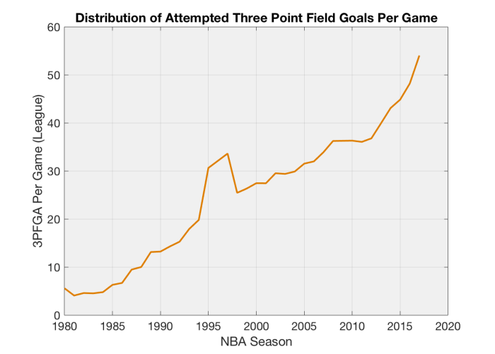
Average number of three point field goal attempts per game over the course of the season. There’s a reason why the spike occurs in the Mid-90’s.
Since 1981, the number of three point attempts per game has been on the rise. Prior to 1985, we would be lucky to see ten total three point attempts in a game. That’s five per team! Thirty years later, we are at nine times that rate at 45 attempts per game. That’s over twenty per team per game.
The graph above displays the rate of attempts per game over the years since the three point line was adopted. There is a significant bump, however, during the 1995, 1996, and 1997 seasons. There’s an extremely simple explanation for this:
In 1979, when the three-point line was adopted, the distance of the line was 23 feet 9 inches from the basket. If we following along this arc, we find that a player would be incapable of shooting from the baseline; as the sideline is a mere 25 feet from the basket. This indicates a shooter must have shoes smaller than 15 inches; a difficult task as a 6’2″ person has roughly 13 inch feet; let alone padding for a shoe. To give the shooter space, a section of the three point line was set to be 22 feet from the basket.
In 1994, the league found that scoring was at an all-time low since the 1970’s with 95 points per game being scored. To combat this, the league moved the three point line to a uniform 22 feet around the basket. Giving shooters an extra 21 inches of three point real estate to launch from. And launch they did, indeed. In fact, the number of three point attempts went from 21,907 in 1994 to 33,889 in 1995 and on to 38,161 in 1996. In 1997, the peak of this craze, we witnessed 39,943 attempts. After the 1997 season, the line was readjusted to its old distances and the number of attempts went back to it’s old progression prior to the shortened distance. In fact, it wasn’t until the 2006 season when the number of attempts in 1997 had been surpassed.
Predicting Three Point Attempts
As we can see, with teams taking 20-25 attempts per game, teams need to find shooters than can convert attempts. Advanced analytics teams collect strong data to build models to predict player capability. For instance, we may collect the distances from the basket a player have taken and ask “How does a player’s field goal percentage decrease as they back up?” If we take game data only, we may ask about other relationships such as “How many shots are contested at the given distances?” or “How does the amount of space and movement of the player leading into an attempt affect their field goal percentage?” These are testable questions; but require advanced data. Some of these questions can be hard to test if only game data is available and the player has a limited number of situations.
Once we have the data we believe will help us answer the questions necessary to piece together for three point field goal estimation, we have to build a model. This model may be complicated, such as graph theoretic techniques or recurrent neural networks. This model may be flexible such as random forests or Monte Carlo simulations. Or models may be simple such as regression models.
For instance, one model I developed years ago (2013) for an Eastern Conference team, leveraged random forests to build a proximity against similar players in the stage of their career. Then, using an ensemble of trained neural networks, the proximities would weight each of the random forests and yield an estimated number of attempts and makes. When applied to Luol Deng, it predicted his decrease but at a slower rate. When applied to Serge Ibaka, it maintained a steady percentage, but refused to ever increase above 2.5 attempts per game. Even if his 4 attempts were included in the model! So complicated models can be fun and taxing; but may not be great.
In this case, we take a look at a regression model. Here, let’s have flexibility… we will run two models to predict the number of misses and the number of makes.
Poisson Regression?
First, let’s assume we have severely limited explanatory data. We have the number of minutes a coach plans to play a player, and the usage percentage of a player for attempts beyond the arc when that player is in the game. These can be dictated by a coaching staff as Deng and Ibaka proven to be with the lead in to this statistical framework.
As we are predicting the number of makes and misses, we have ourselves a counting process. This means we need to use a probability model that puts probabilities on the numbers 0 through infinity. What’s the one everyone learns in undergraduate school? That’s right, the geometric distribution. OK… while that is true, the most common is the Poisson distribution.
Let’s recall the often forgotten meaning of the Poisson distribution. This distribution is used to measure the number of occurrences of an action over a fixed period of time. That is, suppose we have 82 games as our fixed period of time. Then the actions are merely the number of three point makes and misses. We have to make one stingy assumption here that states that all attempts are independent of each other. While this is not so much true; this is not the greatest concern to us.
Now, a Poisson regression model will fit explanatory variables in a manner such that the conditional mean follows a Poisson distribution. That is, if we fix the number of minutes played and the usage of a set of players, the resulting number of three point makes follow a Poisson distribution with mean determined by the explanatory variables. The result of this distribution, however, is that variance is identical to the mean.
So let’s take a look to see if this is indeed true.
2016 – 17 NBA Results
For this past season, we are able to obtain the usage and minutes played for every player in the league. Plotting their resulting makes and misses, we find a nice surface built over these two variables.
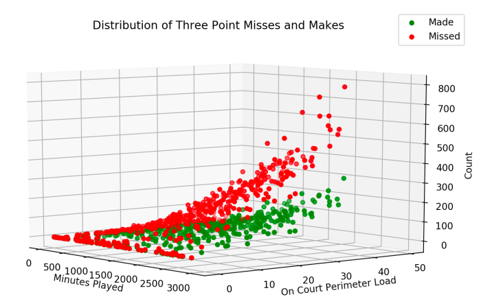
Distribution of three point makes (green) and three point misses (red) for the 2016-17 NBA Season.
As we see the plot, one thing is quite noticeable. We see the increases in the number of makes and misses as a clear function of usage and minutes played. This is obvious to understand. However, we also see the spread of the misses get larger as their usage and minutes increase. At the flatter regions about 500 minutes played and 10-15% usage, totals have averages of 50 and variances of 85. At these high regions, the averages are about 200 with variances of approximately 350. We see immediately that the distribution cannot be Poisson as the variances are inflated compared to the mean. We call this overdispersion.
Negative Binomial Model
The way to incorporate overdispersion in the Poisson model is to enforce a reparameterization. Instead of merely fitting the mean of the Poisson distribution, we can look at the product distribution of the Poisson and Gamma distribution, where the Gamma distribution has a mean of one. What in the world does this mean?!?!
Assume the mean of the Poisson is X. Then, we multiply by a second random variable, say Q, where Q has mean one and is independent of X. Then the reparameterization XQ has the same mean as the Poisson model, but the variance is larger; which is what we need. If you’re in need of technical material for proof, enjoy my hand-written notes…
This resulting model is no longer a Poisson model, but rather a Negative Binomial Regression model. It has mean X but now variance X + a*a*X*X. We see that the variance quadratically increases with the mean; which is what happens in our data!
Apply To The 2016-17 NBA Data
Now we must apply this model to our data. Here I will display the R code associated with fitting such a model. Here, we download the traditional stats for every player last season, as well as the usage stats for every player. We then merge both sets across players to obtain one data set and apply the regression:
library(MASS)
traditional = read.csv(“~/Regression/traditionalstats.csv”)
usage = read.csv(“~/Regression/usagestats.csv”)
allstats <- merge(traditional, usage, by=c(“Player”))
allstats$X3PMiss <- apply(allstats[,c(‘X3PA’,’X3PM’)],1,function(x) {x[1]-x[2]})
allstats$Cross <- apply(allstats[,c(‘MIN.x’,’X.3PA’)],1,function(x) {x[1]*x[2]})model1 <- glm.nb(formula=X3PM ~ X.3PA + MIN.x + Cross, data=allstats, init.theta = 1e-6, control=glm.control(trace=1-,maxit=100))
model2 <- glm.nb(formula=X3PMiss ~ X.3PA + MIN.x + Cross, data=allstats, init.theta = 1e-6, control=glm.control(trace=1-,maxit=100))summary(model1)
summary(model2)results <- cbind(fitted(model1), fitted(model2), model1$y, model2$y)
And here is our output…
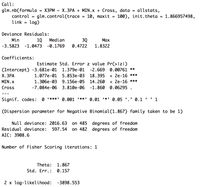
Here we find the fitted dispersion parameter is 1.8667; which is fairly on par with what we witnessed from our raw data. Furthermore, we obtain a model to predict the number of made field goal attempts for a player:
Makes = exp( -0.3681 + 0.1077*USAGE + 0.001306*MINUTES – 0.000007084*USAGE*MINUTES)
Let’s try this out… at least at a basic set-up. Technically, we should leave a sample out to test. So this method below is purely illustrative!
Steph Curry was given 2638 minutes and asked to take 41% of the team’s three point attempts. This results in a predicted number of makes to be 833 made field goal attempts! Yikes! Similarly, we fit for the number of misses. The model is given as:
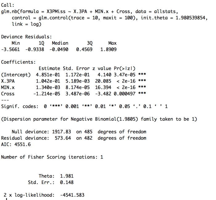
Here we obtain a dispersion parameter of 1.9805, which is also on par with our raw data observations. Understandably, the amount of misses are more varying than that of the makes. For the case of Steph Curry, we have now a predicted number of misses to be 1076 misses! Holy cow…
Despite overestimating Steph Curry’s numbers, we obtain a predicted three point percentage of 43.6462%. This is not too drastic…So why are we obtaining a decent result here? The answer is simple…
Why we predict percentage instead of counts…
The models for both the number of makes and number of misses has so few observations for high volume shooters, as well as some other areas, the variance is going to be dictated by values nowhere near Steph Curry. Hence, the drastic change to go from a Chris Paul to a Steph Curry is actually not as accelerating as going from a Bismack Biyombo to a Chris Paul. In fact, there are more Biyombo-type shooters out there than Chris Pau; and even fewer to get to Steph Curry. In fact there is only one Steph Curry. So we should expect a wildly varying fitted response with such bombastic explanatory variables.
Given these wildly varying changes for sparse amounts of shooters, the nicety for these models are that the shooters are similar between the two sets. Illustratively, Steph Curry makes the most threes, but he’s also at the tops of the lists for missed three’s. Similarly, players who don;t shoot threes will also not make any three point attempts. Combine this with the fact that the variance inflation factors being near similar: 1.8667 for Makes vs. 1.9805 for Misses, we should be able to negate out the inflation differential between makes and misses in three point percentages by simple division.
Results:
Based off our simple set of explanatory variables, we have reasonable predictions for three point percentages. We actually fit decent models. However, the models tend to over-predict for shooters; particularly for shooters who have excessively small number of samples to build off. In this case a zero-inflated model would help compensate for predicting percentages for shooters with zero makes or zero misses. There is a significant amount; we will touch on this in a moment.
One other shooter we cannot account for is Demetrius Jackson (BOS). Jackson was perfect from the field and had a high usage rate of 20% for three point attempts. Given that, his actual minutes were scarce: 17 minutes over five games, four of which were already decided. In other words, Jackson was a garbage time player who managed to make the most of his situation:
- 11 Minutes versus Denver in a 15 point defeat.
- 4 minutes versus Washington in a 25 point defeat.
- 13 seconds versus Golden State in a 16 point defeat.
- 2 minutes versus Orlando in a 30 point victory.
- 11 seconds versus Toronto in a 10 point defeat.
In total, Jackson was 1-for-1; taking 1 of the five three point attempts during his time for that 20% usage rate. Given that we were unable to accurately predict his 100%; we predicted that Jackson is instead a 41.0997% three point shooter; with predicted 1.8057-for-2.5878 three point shooting.
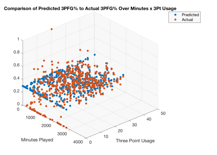
Comparison of Negative Binomial model and actual three point field goal percentages. Zero inflation is in full effect; however it can’t be seen well in this plot. Look at the next one.
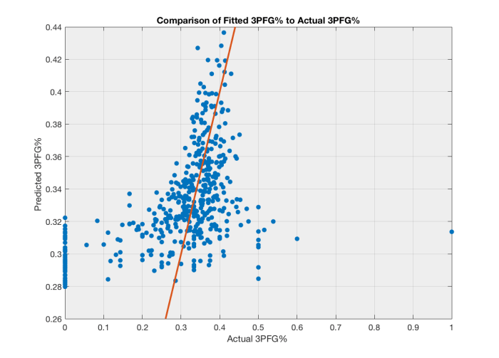
Comparison of predicted 3PFG% to actual 3PFG%. The red line signifies we predicted accurately. Zero inflation is running up the y-axis. Demetrius Jackson is way over on the 100% axis.
In the plots above, we see the predictions as a function of minutes played and three point usage on the team. It’s a little messy, however, we see that shooters who don’t take shots or have missed many of their tiny amount of attempts are pulled up towards the 30% mark. This indicates they are more likely to be 28% – 32% shooters… so keep them at low amount of attempts.
In the lower plot, we see that this biasing is more a function of zero-inflation. Once the zeros are run out; the predicted values tighten up about the red line. The red line, note, is where predicted values are exactly the actual values. Anything to the right of the red line is under-predicting the three point field goal percentage. Anything to the left of the red line is over-predicting the three point field goal percentage. Be very careful to note that the scales on both axes are not the same! It should suffice to include error bounds on the plot. However, setting that up and performing the task is actually fairly difficult as we are performing a transformation on two linear models and if the math hasn’t made you dizzy enough yet; the math of this for surely will. As this will require a transformation on the division of two Poisson-Gamma (Negative Binomial) models with differing inflation parameters.
Conclusions
Here we saw that Poisson regression is ill-suited for predicting three point percentages and that a Negative Binomial model with variance inflation control (NB2 model) is preferable. We also showed that we can fit the model relatively easily if we set the problem up in a nice way to handle counts and applied the model to a basic set of explanatory variables that actually performed not too shabby. Furthermore, we identified the need for zero-inflation handling and identified a way forward for the brave data scientists to forge a methodology for estimating three point percentages in a theoretical and computational manner.
So, what do you think about the process? Try swapping out your own data into the model above an see if you can beat the super-basic model put forth.


Pingback: Basics in Negative Binomial Regression: Predicting Three Point Field Goal Percentages — Squared Statistics: Understanding Basketball Analytics | Advance Pro Basketball