With the Golden State Warriors and Memphis Grizzlies are set to square off for the second time this season tonight, we take an extended look at the most recent 119 – 69 Warrior win over the Grizzlies on November 2nd. We do this by looking at two consecutive possessions that resulted in a Warriors basket and a resulting block from Festus Ezeli on the following Grizzlies possession. The events we break down come from the first quarter with the Warriors leading 17-13 with 4:20 remaining.
Warriors Offensive Possession: Rotate Weak-Side Defense and Slip the Small-Forward
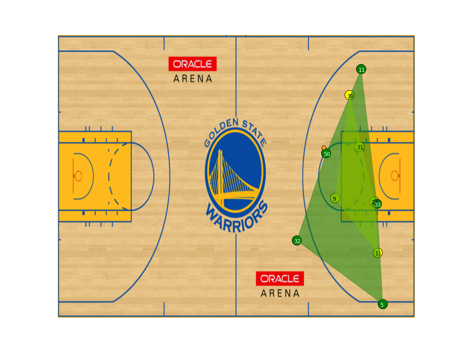
On the Warriors’ offensive possession, Klay Thompson (#11) maintains possession of the ball at the top of the three point arc. After a screen and slip exchange with Draymond Green (#23), Marc Gasol (#5) and Courtney Lee (#33) double Thompson.
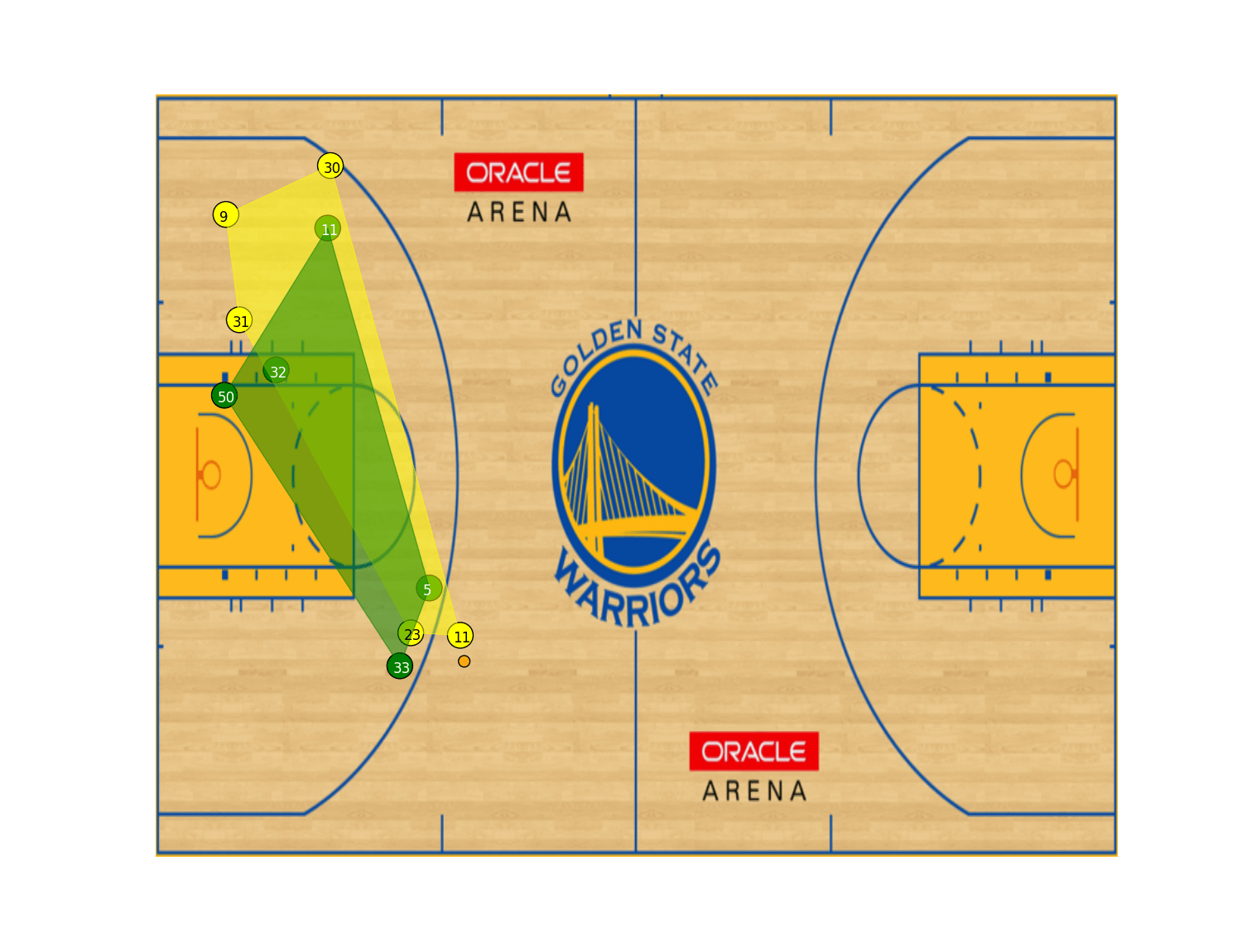
Draymond Green (#23) sets a screen and slip for Klay Thompson (#11).
Thompson passes off to Green, setting up a 4-3 offense at the free throw line. With Steph Curry setting up on the weak-side three point line, there is effectively a 3-2 attack in the lane with no Grizzlies defender on the ball.
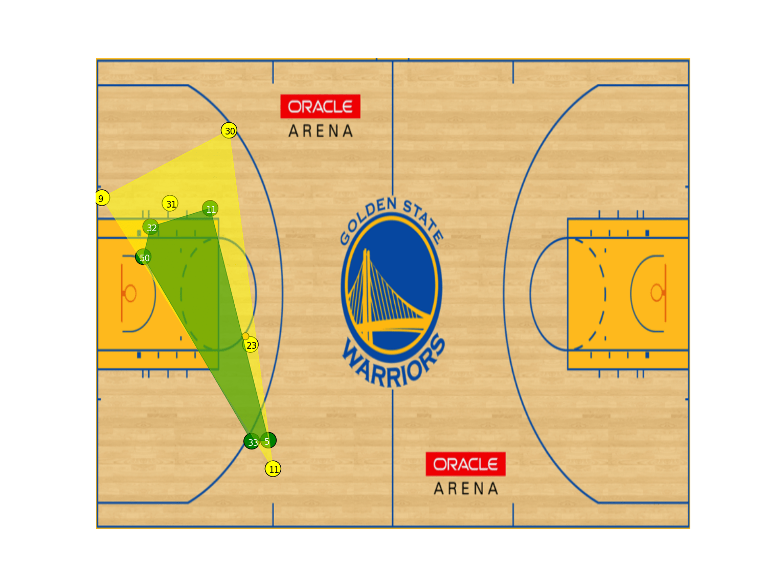
Draymond Green (#23) has the ball at the free throw line, set to attack the basket.
With Zach Randolph (#50) and Jeff Green (#32) caught between Green, Andre Iguodala (#9) and Festus Ezeli (#31), Iguodala slips from the weak-side along the baseline, uncontested. Green hits Iguodala with the pass for the easy two point reverse lay-up.
Draymond Green (#23) hits Andre Iguodala (#9) behind the Memphis Grizzlies defense for a reverse layup.
Grizzlies Ensuing Possession: Rotate Weak-Side Post Over Ezeli for Post-Up
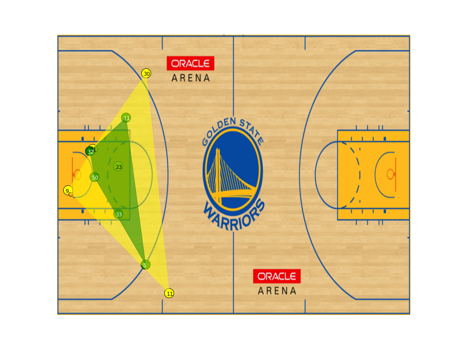
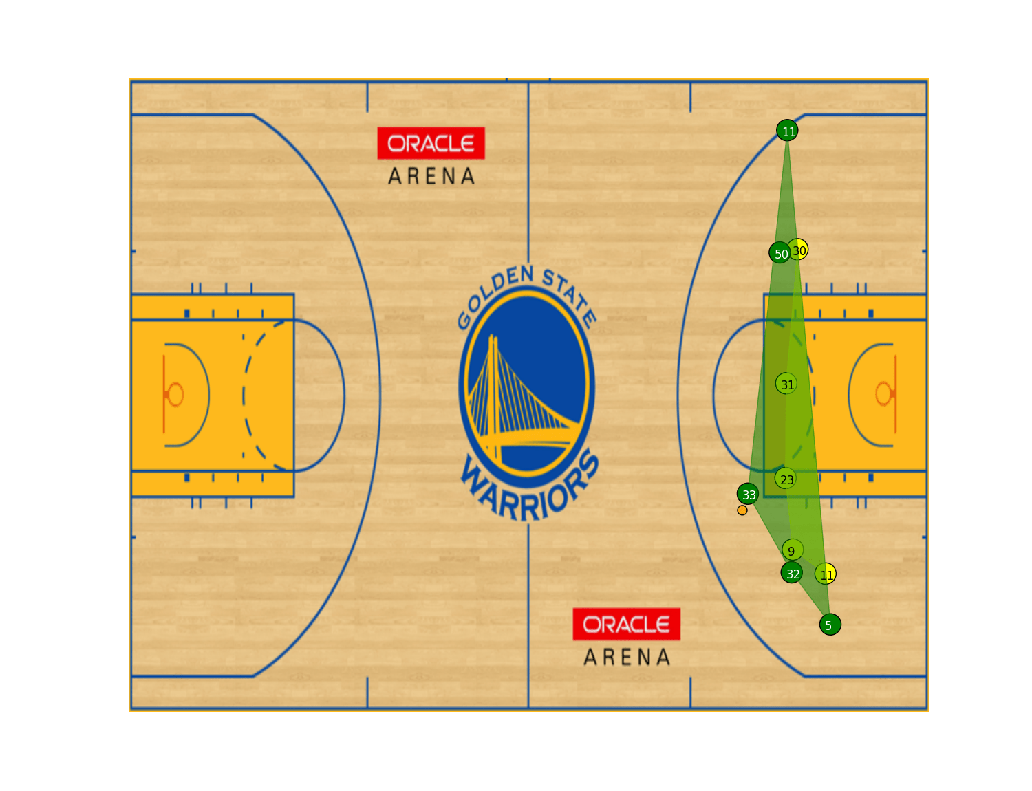
The Grizzlies, in transition, set up in a similar manner with Mike Conley (#11) bringing up the ball on the left side of the court. Randolph (#50) sets the high screen in the same manner as Draymond Green (#23) in the previous possession. However, there is no double team on Conley. Instead, Draymond Green plants himself in on the free-throw line and Festus Ezeli (#31) backs off to the wing, in anticipation of Randolph breaking for the basket.
Zach Randolph (#50) screens Mike Conley (#11) to set up the offense.
Conley dumps the pass off to Randolph in identical fashion to the Warriors previous possession, however Marc Gasol (#33) breaks to the front of the basket. This allows Green to plug the middle, allowing for Green to recover on Randolph. With Jeff Green straying on the three-point line, a 26% three point shooter for the season, Andre Iguodala manages to help pack into the lane without fear of a knock-down three.
Zach Randolph (#50) has possession at the free throw line, but running against a 2-on-3 in the key.
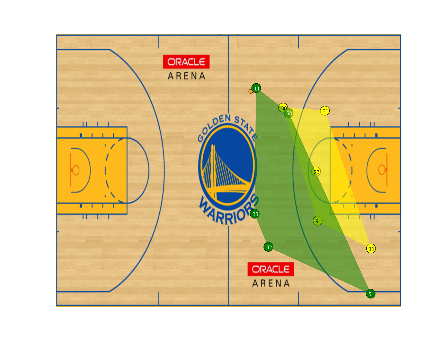
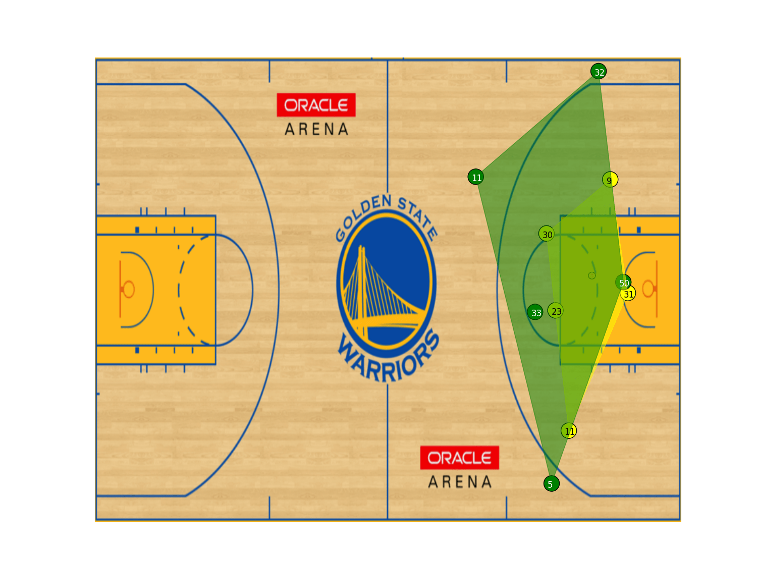
With no easy path for score, Randolph kicks back out to Jeff Green (#32) to rest the offense. Marc Gasol pops out to the high post to allow for a backdoor cut from Green and an exchange for Courtney Lee (#5) to the point. Again, the Warriors defense holds their ground with Festus Ezeli (#31) holding the paint, not allowing the Memphis players to sneak behind the defense.
Marc Gasol (#33) has the ball at the elbow, Jeff Green (#32) makes a backdoor cut, and Courtney Lee (#5) moves to the point.
With a back-and-forth exchange between Gasol and Lee, allowing for Randolph (#50) and Green (#32) to exchange positions to put Randolph on the weak-side block. With a pass back into Gasol at the high post, Randolph breaks from the weak side to post up Ezeli.
Marc Gasol (#33) makes a high-low pass into Zach Randolph (#50) with Festus Ezeli (#31) guarding.
Playing one-on-one with Ezeli, Randolph is unable to make a basket as Ezeli blocks the shot attempt with a 1.04 seconds remaining on the shot clock. The moment ends as Festus Ezeli is subbed out for Mo’ Speights; and Zach Randolph, Courtney Lee are subbed out for JaMychal Green and Matt Barnes.
Animation of the Two Plays
We can string together the images to form an animation of the distribution of the defenses using any tools at our disposal. For the two plays broken down above, we obtain the following animation:
Using Python to Break Down Plays
To extract data and build the models, we write a basic Python file. First, we make our library calls to have some necessary functions at our fingertips.
import requests
import pandas as pd
import numpy as np
import matplotlib.pyplot as plt
from scipy.spatial.distance import pdist, squareform
from scipy.spatial import ConvexHull
import csv
import matplotlib.image as mpimg
Using the requests and pandas libraries, we will make a call to a server that contains JSON files containing NBA tracking data. The numpy and scipy library imports will give us the ability to build data arrays that we can apply some of the convex hull mathematics once we extract out the JSON file data into a manageable data set that we can use for many different applications. Finally, we import the matplotlib libraries to display the results as tidy visualizations.
Next, we want to extract the data by contacting a publicly available server by setting the url as a variable and making a request to the server for the JSON files.
url = “http://stats.nba.com/stats/locations_getmoments/?eventid=78&gameid=0021500051”
response = requests.get(url)
response.json().keys()
home = response.json()[“home”]
visitor = response.json()[“visitor”]
moments = response.json()[“moments”]
The url is located on stats.nba.com. Here, we must submit a request with a game_id and an event_id. The game id is 0021500051. This value means we are in season 002150 and game number 0051 of 1230. The event id is a period of time defined by stats.nba as a sequence of moments from the game. In this particular instance, event id has a total of 836 moments, which is the two full possessions for each team. In the above analysis, we only used the first 781 moments, since there are three substitutions for the final two seconds of the event id.
The resulting request accesses the JSON file, where we can break out the team dictionaries and the moments of the event. We can set the dictionaries by using the home, visitor, and moments requests. This loads a series of tables that are readable by pandas. The contained data can be understood by a previous post.
headers = [“team_id”, “player_id”, “x_loc”, “y_loc”, “radius”, “moment”, “game_clock”, “shot_clock”]
player_moments = []
for moment in moments:
for player in moment[5]:
player.extend((moments.index(moment), moment[2], moment[3]))
player_moments.append(player)df = pd.DataFrame(player_moments, columns=headers)
We then set the headers in accordance to the moments vector in the JSON file and set a player_moments table. The value moment[5] is the collection of the 10 players and basketball for the given time in the game, indicated by period in moment[0], and time remaining in the period, indicated by moment[2].
For each moment, we pull the 11 players and extend the vector by adding the time remaining in the quarter and shot clock time remaining. We then append this extended vector to the player moments vector. The resulting data frame combines the player_moments with the headers, so we can take a good look at the data. As an example, using the command print df.head(11) prints the first 11 entries with the respective columns; one for each player and the basketball.
players = home[“players”]
players.extend(visitor[“players”])idd = {}
for player in players:
idd[player[‘playerid’]] = [player[“firstname”]+” “+player[“lastname”],
player[“jersey”]]idd.update({-1: [‘ball’, np.nan]})
df[“player_name”] = df.player_id.map(lambda x: idd[x][0])
df[“player_jersey”] = df.player_id.map(lambda x: idd[x][1])
Next, we build a dictionary of players that maps the player_id number to the player names and jersey numbers. The data frame is then mapped with the player name and jersey numbers. Next, for our particular purposes, we build a csv file that can be used by many different mediums. To do this, we break each player from the event file.
Iguodala = df[df.player_name==”Andre Iguodala”]
Curry = df[df.player_name==”Stephen Curry”]
Ezeli = df[df.player_name==”Festus Ezeli”]
Thompson = df[df.player_name==”Klay Thompson”]
dGreen = df[df.player_name==”Draymond Green”]
Randolph = df[df.player_name==”Zach Randolph”]
jGreen = df[df.player_name==”Jeff Green”]
Lee = df[df.player_name==”Courtney Lee”]
Conley = df[df.player_name==”Mike Conley”]
Gasol = df[df.player_name==”Marc Gasol”]
ball = df[df.player_name==”ball”]outdir = ‘/homefilelocation/’
outfile = open(outdir+”GSWvMEMTwoPlays.txt”,’a’)
for i in range(782):
outfile.write(str(i+1)+’,1,’+str(Iguodala.player_jersey.iloc[i])+’,’+str(Iguodala.x_loc.iloc[i])+’,’+str(Iguodala.y_loc.iloc[i])+’\n’)
outfile.write(str(i+1)+’,1,’+str(Curry.player_jersey.iloc[i])+’,’+str(Curry.x_loc.iloc[i])+’,’+str(Curry.y_loc.iloc[i])+’\n’)
outfile.write(str(i+1)+’,1,’+str(Ezeli.player_jersey.iloc[i])+’,’+str(Ezeli.x_loc.iloc[i])+’,’+str(Ezeli.y_loc.iloc[i])+’\n’)
outfile.write(str(i+1)+’,1,’+str(Thompson.player_jersey.iloc[i])+’,’+str(Thompson.x_loc.iloc[i])+’,’+str(Thompson.y_loc.iloc[i])+’\n’)
outfile.write(str(i+1)+’,1,’+str(dGreen.player_jersey.iloc[i])+’,’+str(dGreen.x_loc.iloc[i])+’,’+str(dGreen.y_loc.iloc[i])+’\n’)
outfile.write(str(i+1)+’,2,’+str(Randolph.player_jersey.iloc[i])+’,’+str(Randolph.x_loc.iloc[i])+’,’+str(Randolph.y_loc.iloc[i])+’\n’)
outfile.write(str(i+1)+’,2,’+str(jGreen.player_jersey.iloc[i])+’,’+str(jGreen.x_loc.iloc[i])+’,’+str(jGreen.y_loc.iloc[i])+’\n’)
outfile.write(str(i+1)+’,2,’+str(Lee.player_jersey.iloc[i])+’,’+str(Lee.x_loc.iloc[i])+’,’+str(Lee.y_loc.iloc[i])+’\n’)
outfile.write(str(i+1)+’,2,’+str(Conley.player_jersey.iloc[i])+’,’+str(Conley.x_loc.iloc[i])+’,’+str(Conley.y_loc.iloc[i])+’\n’)
outfile.write(str(i+1)+’,2,’+str(Gasol.player_jersey.iloc[i])+’,’+str(Gasol.x_loc.iloc[i])+’,’+str(Gasol.y_loc.iloc[i])+’\n’)
outfile.write(str(i+1)+’,0,0,’+str(ballz.x_loc.iloc[i])+’,’+str(ballz.y_loc.iloc[i])+’\n’)outfile.close()
This block merely iterates through each of the players and writes a time sequential file that contains: time_id number, team_number (1, 2, 0), player_jersey_number, player_x_loc, player_y_loc. Ideally, we can pass this to a matrix using np.array. Instead, we saved the write off for use in programs such as MATLAB and C. So we will proceed as if the files already exist.
inFile = outdir + ‘GSWvMEMTwoPlays.txt’
with open(inFile,’r’) as dest_f:
data_iter = csv.reader(dest_f,
delimiter = ‘,’,
quotechar = ‘”‘)
data = [data for data in data_iter]data = np.array(data,dtype=’float32’)
N = data.shape[0]
Here, we read in the text file using csv reader and put the resulting five-column matrix into a numpy array. We then break out the number of images we will construct.
M = P.shape[0]
mm = M / 11
Finally, we call for the convex hull for each moment and plot onto an image of the Warriors basketball court.
plt.ion()
figg = mpimg.imread(‘/FileLocation/WarriorsCourtF.png’)
for i in range(mm):
players = P[11*i:11*(i+1),2].astype(int)
labels = [‘{0}’.format(j) for j in players]
points_defense = P[11*i:11*i+5,3:5]points_offense = P[11*i+5:11*i+10,3:5]
hulld = ConvexHull(points_defense)
hullo = ConvexHull(points_offense)plt.figure(figsize=(15, 11.5))
plt.imshow(figg, zorder=0, aspect = ‘auto’, extent=[0,94,50,0])
plt.fill(points_defense[hulld.vertices,0], points_defense[hulld.vertices,1], fill=True, color = ‘yellow’, alpha = 0.5, edgecolor=’yellow’)
plt.fill(points_offense[hullo.vertices,0], points_offense[hullo.vertices,1], fill=True, color=’green’, alpha = 0.5, edgecolor=’green’)plt.scatter(x = P[11*i:11*i+5,3],y = P[11*i:11*i+5,4],marker=’o’,c=’yellow’,s=500)
for label,x,y in zip(range(5),P[11*i:11*i+5,3],P[11*i:11*i+5,4]):
plt.annotate(str(labels[label]),xy=(x-0.5,y-0.5),color=’black’)
plt.scatter(x=P[11*i+5:11*i+10,3],y=P[11*i+5:11*i+10,4],marker=’o’,c=’green’,s=500)
for label,x,y in zip(range(5,11),P[11*i+5:11*i+10,3],P[11*i+5:11*i+10,4]):
plt.annotate(str(labels[label]),xy=(x-0.5,y-0.5),color=’white’)
plt.scatter(x=P[11*i+10,3],y=P[11*i+10,4],marker=’o’,c=’orange’,s=100)
plt.axis(‘off’)
plt.xlim(0,94)
plt.ylim(0,50)plt.draw()
changer = ‘%03d’ % i
plt.savefig(‘/FileLocations/GSWvMEM’ + changer + ‘.png’)plt.clf()
Here, the convex hull is already defined via scipy, so there is little work to do. Most of the work is extracting out the 11 positions, listing out which five are offense, which five are defense, and which is the basketball. Once we have that, everything else is done using an matplotlib.
First, we plot the points on the Warriors court. This is done by using the scatterplot function and plotting large enough circles that will contain the player jersey numbers. Next, we apply the annotate function to put the respective jersey numbers onto the circles. We then cap off the scatterplot by using the fill function to color in the convex hull obtained.
Printing each image off, we have a directory of images from the two possessions; each respective of their moments. Here we can either call the animation library and build an animation, or we can simply upload the videos into our favorite video animation tool.


Pingback: Identifying Player Possession in Spatio-Temporal Data | Squared Statistics: Analyzing Crime, Sports, and People