One of the challenges in data science within the NBA is diagnosis. Diagnosis is the process of collecting and dissecting data in an effort to reveal and understand the components of such data such that we can extrapolate intelligence. Within many NBA analytics circles, this is done heuristically: discussion of a question, hypothesizing new variables, and then quantifying said variables. Unfortunately, without care, this system is flawed due to confounding of lurking variables. Take for instance…
Question: Who is an “elite” paint defender?
Heuristic: Measure three variables: Field goal percentage in paint, Field goal frequency in paint, Rate of passes out of paint after player drives/cuts into paint.
This isn’t a terrible set-up. The thought process is rather direct as it focuses primarily on end-state results. It’s an analysis that helped idealize Roy Hibbert several years ago. And while Hibbert was a great interior presence, his numbers are rather confounded: his Defensive Rating was only at “elite” levels when effectively both Paul George and David West were on court. More importantly, the pressure Hibbert yielded on the interior, combined with the pressure of the guards and other Bigs led to teams taking less efficient field goal attempts.
(Side Note: When I was working with an Eastern Conference team, the lead analyst mentioned he would have rather taken Hibbert over Blake Griffin if given the opportunity. The following year, Hibbert went to LAL and I made the bet that Hibbert’s defensive numbers would decrease dramatically over the next couple years because he doesn’t have D. West next to him anymore. The comment was tongue-in-cheek and West was emphasized as George had missed the year due to the leg injury, but the numbers did drop and has widely been blamed on the shifting tides of the NBA.)
Instead of making this an article about Roy Hibbert, let’s focus on the shifting tides that were becoming clear: Teams were finally adopting long range approaches and more complex offensive schemes to force rim protectors away from the rim. This led to sequences such as Hammer attacks or “Screen-the-Screener” action that would intentionally tangle rim protectors.
From a data science perspective, this becomes a nightmare in confounding players versus the system, IE: the Jae Crowder problem. The drives that result in a pass away from the basket? Are those designed passes to find open players within a complex offensive scheme or because the rim protector is a legitimate rim protector? The low frequency of rim two’s? Is this a fact that the team is finding a dynamic motion to to open more three point attempts? Here, we begin to understand the need for a random effects model that begins to separate out the system, which is widely considered a lurking variable for measures such as BPM and RAPM, from the player. In this article, we start to look at identifying the system.
Random Effects: Turning the Lurk into a Feature
The challenge with constructing a lurking variable into a feature is due to the inability to measure the lurking variable accurately. For measures such as Player Efficiency Rating, Box Plus-Minus, or Regularized Adjusted Plus-Minus, the values are derived from play-by-play data or synthesized from box score data; without any ability to adjust for play type. This play type (system) becomes effectively the reason a player such as Jae Crowder performs well for a 50+ win team in Boston that cannot escape the Eastern Conference Playoffs but then struggles mightily with a 50+ win team in Cleveland that eventually makes the NBA Finals. To this end, these types of models are effectively Y = g(f(X)), where Y is the resulting measure, X is the player activity, f is the function that measures the player, and g is the noise model. For RAPM, this model is explicitly given here. In a primitive form, the model is given by
Rating = Player on Court + Error
This model is effectively a first order random effects model. The first order means that the model only looks at the variables measured and no interactions. If RAPM truly cared about pairs of players, we’d see the explosion of variables where the 1’s and 0’s are multiplied. In this case we don’t, and we are left with a first order model. The randomness comes from not being able to define what players are one the court. Instead, we just sample them as they come. This is different than a fixed effects model, where we can simply identify who is playing when before the entire games begins.
Our goal at this point is to impose a new feature: the play type. We can then look at the model
Rating = Play Type + Player on Court + (Play Type x Player on Court) + Error
and we have ourselves a second order random effects model. We can visualize the play type as a grouping or treatment in terms of designs of experiments; but this now requires us to cluster play types; and hence measure the lurking variable. And there are two ways to do this: Mechanical Turk or Tracking Data.
Mechanical Turk
The Mechanical Turk is a method of developing labels by hand instead of machine. It’s name comes from the famous chess playing “machine” from 200+ years ago. It is also the primary method for Synergy and Krossover data collection. The process is tedious and often flawed. If you haven’t heard the question “Is that really a PnR?” 1000 times when working with Synergy, you haven’t worked with Synergy data enough. However, the process is good enough to produce actionable labels.
The PnR question from above started to make a lot of problems for analytics departments when the question if whether a hip tap by a passing by “screener” or an unused “screen” of a “screener” 5+ feet away from the play were considered as pick-and-rolls (even shallow cuts were being labeled as PnR’s).
While the simple understanding of identifying a screen becomes a challenge, more complex schemes such as breaking out plays becomes a near impossible task for these methodologies. For starters, to break down a play in the NBA we typically need to at least see the play three times. And that’s for experts who can break plays down.
Tracking Data
Tracking data instead allows the scientist to apply machine learning techniques to help tease out actions. In this case, we are able to template plays based on their spatio-temporal patterns and then cluster the actions. And while this may seem sexy and time saving; this process if too often flawed. If you’ve ever heard the question “Is that really a post touch?” enough times when working with Second Spectrum markings data, then you haven’t worked with enough Second Spectrum data. Notice a trend here?
Regardless, attempting to identify complex plays using tracking data is also a very difficult task. There have been some public attempts, such as sketching from Andrew Miller; which performs a segmentation of track paths made by players, a functional clustering of segments (treating components as words), and modeling possessions (treating possessions as a topic modeling problem).
It’s a fairly strong attempt, and is fairly on par with my work since interacting with SpotVu data with teams from many seasons ago. However, this methodology suffers from the dreaded time-warping problem. That is, players run at different speeds along fuzzy paths in the same direction due to either competency or design. Taking a look at Miller’s paper above, time-warping rears its ugly head when cuts or perimeter motion takes effectively between 2 and 8 seconds.
A key benefit to the procedure, and why it becomes such a strong attempt, is that this is an unsupervised technique; allowing for construction of plays without encoding plays. Along with this unsupervised formulation, interpretability is easily available as tracks are identified as the vocabulary.
Tensor Approach
The methodology I’ve been using for the better part of five years comes from development on SportVU data with that same aforementioned Eastern Conference team. When it was originally presented to the staff, I probably received the largest glassy-eyed response I’ve ever received in my life. But at the end, it was able to separate out the effect of the defensive system on a player such as Roy Hibbert and identify that he was a product of the system; which maximized his talents exceptionally well. And, unfortunately, it’s not as a visually cool application as Andrew’s work above.
The methodology is rather tedious: We start with a collection of unmarked plays and break out their locations at each time step as a binned structure; not much unlike the shot locations in the Nonnegative Matrix Factorization procedure for field goal attempts. From there, we have to identify that we are now victims of two types of alignment: play start alignment and time-warping.
For play start alignment, we employ a Fast-Fourier Transform, treating the position of the players and the basketball as a a signal over time. The resulting power spectrum can be used to cross-correlate plays to identify differences in start times between two similar plays in the 2D Fourier spectrum. Consider this equivalent to comparing two arbitrary signals over time that end up being same frequency, same information content with noise, disrupted by a time-delay. If the cross correlation’s peak is at time zero, the signals are at the same time. If the peak is offset from zero, the offset is the play alignment. The width of the cross-correlation is two-fold: “flat” schemes are differing plays and “fat” schemes are similar plays with time-warping or players doing slightly different actions. Unfortunately, identifying peaked cross-correlations doesn’t help us much; unless we mechanical turk plays in advance and use them as templates. And even then, this is a global property. Any slight changes will flatten and fatten the cross-correlation and leave us with no immediate reason as to why.
For time-warping, we tackle this problem later.
So let’s start understanding this system through the use of a particularly well known strategy: the Horns structure. Under this set-up, we will start to break down different Horns plays and apply data science techniques to uncover features that break the plays down.
Horns Twist
The Horns offense is a well-known offense that is initialized with a dual screen action towards the ball handler. The “Twist” action is when the ball-handler is screened twice. Once by each screener, leading to a zig-zag pattern.
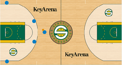
Typical starting pattern of Horns.
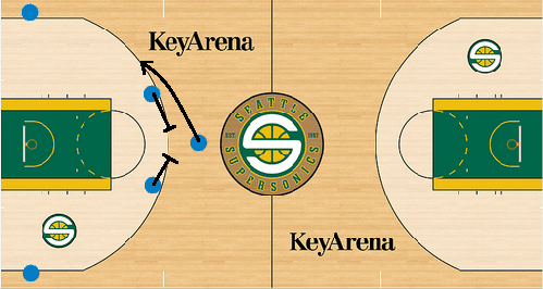
Dual screen action with ball-handler going right.
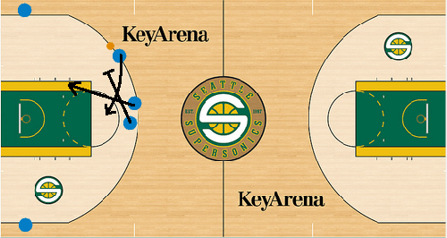
Screener rolls to allow other initial screen man to “Twist” the ball-handler.
The action is straightforward and commonly used to tangle interior defenders at the free throw line. This will either open up a driving mismatch for the point guard 12-15 feet from the rim, open up a pullup three point attempt from the top of the key, or open up the initial screener underneath the rim.
To illustrate out process, we take a sequence of five Horns Twist plays to the right and plot them on the court. These plays have been subjected to the FFT mentioned above and the play tends to look very predictable.
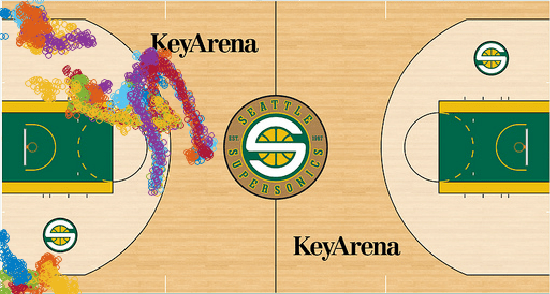
Collection of five FFT’d Horns Twist Actions to the Right.
If we up this towards twenty five samples, it begins to take a life of its own.

Collection of 25 FFT’s Horns Twist Actions to the Right.
And now we start to see the jumbled mess we expected to see. Don’t ask for 500 of them, it colors almost a third of the court. However, we are able to start mapping out the tensor over time:

Check it out: The tensor of 100 convolution-adjusted Horns Twists plays to the right. If you ever hear me mention WORMHOLE, this is the plot I’m referring.
Tensor Decomposition
Applying a tensor decomposition, we start to identify characteristics, or signatures, of different styles of play. Here, we apply a nonnegative CANDECOMP-PARAFAC decomposition. This allows us to start breaking down the plays into a number of components.
For instance, if we settle on one component to represent a Horns Twist, we end up with a Sideline component, a Baseline component, and a Temporal component:
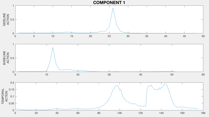
Here is the Single Component Decomposition of the Horns Twist to the Right action.
The sideline action will capture components of motion that occur along the sideline. Similarly, baseline action captures motion along the baseline. The temporal component identifies the segments of when activity occur. To reconstruct the play, we focus on the outer-product of these components. By taking the outer product, we see a significant amount of activity happening at the right of right around the perimeter. This component captures the motion of the screens and the ball-handler. In this case, the non-moving shooters have relatively insignificant roles; despite the small blips at 1 and 50 in the Baseline action; and the small blip at 1 in the sideline action.
More importantly, in the temporal component, we identify the screen actions. The first bump is the first screen, the second bump is the screener chasing the ball-handler and the second screen being set. The slight dip is the second screener approaching the ball-handler.
More Components = More Actions…
If we wish to expand on the decomposition and focus on breaking out particular components, we can. However, it should be noted that more components does not necessarily indicate better fit. In fact, if we break down the Horns Twist play with five components, we get seemingly more actions:

Rank five decomposition yields five “components” of action. But is it really action?
Here, we immediately see our rank-one action as the first component in the tensor decomposition. But now we see other activities. What is component 2 capturing? This happens early on in the possession, and again late. It’s location is primarily focused near the center of the court. Similarly, there’s two primary actions in accordance with the sidelines: This is effectively the initial screener’s role. In fact, this is his screen action towards the ball handler and subsequent roll to the basket. The temporal component at the end is the motion of the ball-handler entering into this region after the second screen.
Component three trims on this exact same action, allowing us flexibility in modeling the pick and roll type action that occurs on the first screen. What ultimately happens is that the collection of these components captures players’ roles and motion within an offensive scheme. For a common possession, I tend to use fifty components.
Side Note: There’s no distinct tried and true way to select the optimal number of components. This is an actual open research problem. Fifty is just a feel-good, warm, fuzzy number.
Time Warping…
Alas, that time warping problem is back. Here, we mitigate it by using a dual attack on the temporal component. Using the tensor decomposition, the motion of the players will elicit similar signatures. However, we will see changes in the temporal components associated with the motion. A slow player will have distorted temporal changes. A delayed player, will have a shifted temporal component.
At this point, we again appease to the Fourier transform gods and cross-correlate these signals to find speed/reaction of player (fattening) and strategic delay (offset).
Let’s take a look at a subtle wrinkle.
Horns 4-5
The Horns 4-5 play is a near identical action as the Horns Twist play. The exception is that the secondary screener screens the primary screener.

Same initial set-up as Horns Twist.

However, a screen the screener action occurs.
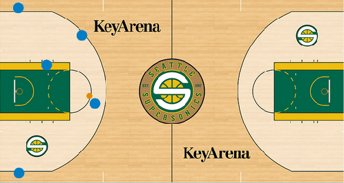
Which can turn into a shot at the top of the key for the primary screener.
This secondary screen action frees the original screener and typically sets up a three point attempt, or forces the interior defender to step up, freeing the secondary screener to slip into the lane. In this case, we selected 25 FFT’d pops:
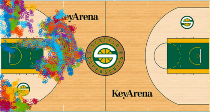
Capture of 25 Horns 4-5 pop players that went to the right.
And the associated wormhole plot:
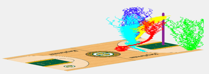
Wormhole plot of a Horns 4-5 to the right with a pop action.
As we start to break down the components, we immediately see a different structure. For a single rank-1 decomposition, we obtain a seemingly significantly different result:

Rank-1 Decomposition of the Horns 4-5 action.
We see the two screens like before, but this time they are located in different spots. We see the identical screen set at roughly 12 feet along the baseline and about 20 feet out from the basket. However, we see the second screen action that short of the first. This is the staggered screen the screener action. We also pick up the resulting flare of the primary screener as the rolling drop of the baseline action.
Similarly, the temporal aspect shows that the Horns 4-5 acts as a “smoother” play as two screens can interact simultaneously; as opposed to the Horns Twist that requires a staggered time-delay screen on the ball-handler.
Expanding out to five components, we have a similar decomposition of the play:
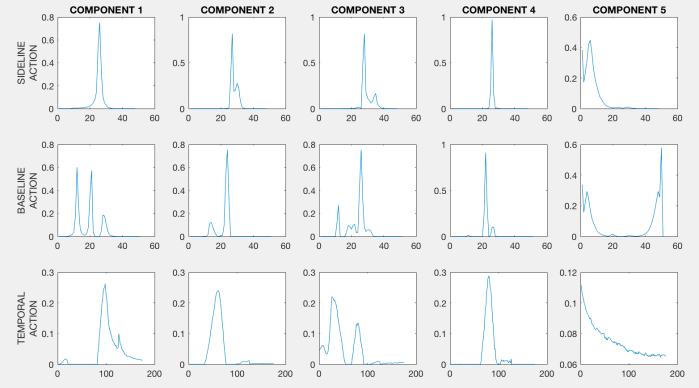
Rank 5 decomposition of the Horns 4-5 action.
Comparing these components to the Horns Twist components, we start to see the massive differences between the two plays in the decomposition space.
Templating Plays
At this point, we have to make a decision: do we store templates or use an autonomous structure. The former action resorts back to a mechanical Turk type activity. Here, we use subject matter expertise to design out plays and then collect the plays to diagnose a signature. Instead of keying thousands of plays; we merely have to key approximately 200 plays and use the template going forward. More importantly, we can diagnose specific actions within a play; and diagnose those. Typically, we piecemeal actions together.
The latter is to aggregate all actions and perform a decomposition with a large rank; or large number of components. This allows us to not have to template, but requires a significant amount of tender, love, and care to tease out actions and label them. This is more in the flavor of Miller’s paper above, but potentially runs the risk of developing many false-positives: ghost actions that don’t really occur but reduces the noise in the observed tensor.
Despite this, we can then take a team’s actions and merely fit the components to a team. This will yield a collection of coefficients that in turn. These coefficients acts as weights for the types of plays that teams run. For instance, in the 2015-16 NBA season, the highest weight for the Los Angeles Clippers was the Horns 4-5. This play, coincidentally, was a Bread-and-Butter play for the Clippers when ran with Chris Paul, Blake Griffin, and DeAndre Jordan. Furthermore (not so coincidentally), when Austin Rivers replaced Paul, the timing was significantly flattened out; indicating that the play took much longer to develop.
It’s indeed a heavy-lifting methodology; but it’s a way for data science to interact with NBA modeling by leveraging tracking data without having to impose heuristically developed features that can be tainted by lurking variables.
Pingback: Weekly Sports Analytics News Roundup - October 23rd, 2018 - StatSheetStuffer