In the era of possession-based statistics, we often look at items such as per-possession or per-100 possessions. This type of parsing makes sense as a possession is deemed to be the period of time a team “controls” the basketball. The technical definition of a possession defines the end of the “control” period as the point of time when the defense has secured the basketball to start transition into offense or the period of play has expired. However, when we start to break down possessions, things get a little wonky.

Pelicans – Timberwolves: 30,000 Foot View

For instance, let’s take a look at the New Orleans Pelicans and the Minnesota Timberwolves from last season. Both teams finished with a 111.4 offensive rating and slightly different defensive ratings: 112.6 (Pelicans) to 112.9 (Timberwolves). From a casual level, we’d expect these teams to end up roughly the same in the standings, as they are both from the same conference. And to a degree, that’s effectively what happens. The Timberwolves finished the year at 39-43 while the Pelicans clambered in at a Zion-winning 36-46.

Despite these ratings, we barely have scratched the surface with these two teams. For starters, the Pelicans played in roughly 220 more possessions than the Timberwolves: 8497 to 8279 on offense and 8504 to 8278 on defense.  This suggests that the Pelicans played at a faster pace than the Timberwolves. And this is indeed the case at the topical level where the average possession for the Pelicans is 13.94 seconds (3rd in the league) to the Timberwolves’ 14.37 seconds per possession (14th in the league).

Remember, these teams have identical offensive ratings. Therefore, combined with adjustments for pace, we should see the same distribution of potential offensive possession ending categories: Field Goal Attempts, Free Throw Attempts, and Turnovers. Here, we make the assumption that end of period possessions are negligible as teams tend to have nearly identical amounts of period ending possessions.

In this case, we find that the Pelicans 140 extra turnovers compared to the Timberwolves, but 74 less free throws. That’s an estimable 107 extra possessions from the Pelicans. We expect, if all extra field goals are misses with defensive rebounds, the Pelicans to have roughly 110 extra FGA’s as a best case scenario for breaking down an offensive possession. Instead, we find that the Pelicans have a measly 80 extra FGA’s. This means we are missing 30 possessions when comparing these teams…

The reason for this, is due to the chance. 

Chance: The Units that Make Up a Possession

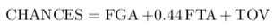
A chance is defined to be a segment of a possession that results in a field goal attempt, a free throw attempts that results in a potential change of possession, or a turnover. It is the segment of time that breaks up a possession into actions that result in loose balls (rebounds) or outright change of possession (out-of-bounds, steals). Every chance, like a possession, has a point value attached to it. And a nice relationship of possessions and chances is given by

From this relationship, we can model possessions as a collection of chances. Using chances, we can start to decompose players into their roles within a chance. While we understand that all possessions are not equal, chances are also not equal. Back in May, we took a look at the impact of turnovers on possessions/chances; in both dead ball and live ball situations. Four months later, Seth Partnow took a more in-depth look at the typical “five” categories for ending possessions:

1. Live Ball Turnovers (steals)
2. Defensive Rebounds on Missed FGA’s
3. Dead Ball Situations
4. Offensive Rebounds
5. Munged Category of FGM’s, FTA’s, and DREBS on FTA’s.

These categories are almost a perfect partitioning of points. Steals lead to zero points on offense. Dead Ball situations are effectively dead ball turnovers with zero points on offense. Defensive Rebounds on Missed FGA’s are zero points on offense. However, Offensive Rebounds are not necessarily pointless chances, as they may come off of missed FTA’s after a basket (and-1) or a missed back-end of FTA’s. We make this note to identify that the category that deserves the most care in analysis of chances is the offensive rebound.

In particular, it is this category quantity that drives the well-known Second Chance Points statistic. And it is here that Minnesota “steals” possessions away from New Orleans in the comparison above.

Timberwolves Taking Some Chances

Taking a step back from Seth’s “five” categories, traditionally, a chance has been defined as through field goal attempts, free throw attempts, and turnovers. Traditionally, from box score data, the number of chances has been represented as

We parse this down as a field goal attempt will lead into one of four results: a defensive rebound, an offensive rebound, a transfer of possession due to made field goal, or a free throw attempt due to foul. Through free throw attempts, obtained either through continuation or non-continuation, is traditionally viewed has having a forty-four percent chance of transferring possession to another team through made free throw, becoming a defensive rebound, or staying with the offense through an offensive rebound. There are other nuanced situations with free throws, but we will deem them negligible; such as the free throw that results in turnover due to lane violation on the offense.

Using this traditional setting, we find that the Timberwolves attempted 9,435 chances compared to the Pelicans’ 9,570; a difference of 135 chances. While this doesn’t explain the full 30 possessions that seem to be missing, we find out that the Timberwolves had more offensive rebounds and therefore had more opportunities to score per possession than the Pelicans.

Given a Chance, Let’s Talk Usage

With the notion of chance outlined above, the real goal of this article is to identify subtle artifacts of team dynamics. For instance one year, while working for an Eastern Conference team, I was out scouting a college game with another analyst. During the game, the analyst mentioned something about how three 25% usage players cannot coexist on the same team because their usages are too high, there’s only one ball.

I mentioned that usage cannot be added as it’s a ratio. I was told, “Usage is not a ratio. Usage is usage.” It was a very alarming comment to hear, especially from an analyst on a team. But none-the-less, I retorted that all probabilities must sum to one in the end. Unfortunately, I was scoffed at over the notion that probabilities had to add to one…

Despite the pushback, the traditional form of usage is a ratio of chances completed by a player given the number of chances possible during the player’s time on the court. The current standard model for usage is given by

There is an abuse of notation here, but we will explain it. The value P is the player of interest, while Pt is the time at which a player is on the court. This means the numerator is the number of chances executed by a player, while the denominator is the number of chances executed by the team while the player is on the court. The resulting value of usage is then a percentage of chances executed by the player, P. Commonly this value is multiplied by 100 to help readers understand that it is a percentage.

The above formula is the classic play-by-play version of usage. In the box-score version, adjustments using minutes played and a factor of five emerges to estimate the denominator. This is exactly the form found on basketball reference.

What is not so well established is that usage is a conditional statistic, dependent on a sampling frame. This means, usage has to be treated with care when being discussed. Making claims about two 25% usage players is almost completely meaningless if they are not sampled using the same sampling frame.

In the end, chances have to be gobbled up by players and ultimately someone on a team will gobble up over 20% of chances. Let’s take a look at this over a simulation…

Example: 2-on-2 Game

Consider a game of 2-on-2 with teams of 4 players. In this case, there are six potential lineups. If players are labeled A, B, C, and D; the lineups are labeled as AB, AC, AD, BC, BD, and CD. Suppose we witnessed 1000 chances played by this team and they have the following breakdown:

• Lineup AB: 300 chances
• Lineup AC: 200 chances
• Lineup AD: 200 chances
• Lineup BC: 100 chances
• Lineup BD: 100 chances
• Lineup CD: 100 chances

Also suppose there is a secret true underlying usage of each player. That is, there is a real probability that a player would complete a chance given across the team. This probability must add to one across the team. Using this true underlying usage probability, we can then simulate chances and obtain an observed usage value.

Note that from this rotation, A plays in 700 chances, B plays in 500 chances, C plays in 400 chances, and D plays in 400 chances. Running one simulation, we find that the usage for each player is given by (.801, .404, .410, .1825), for players A, B, C, and D, respectively. This is obtained from the usage formula above!

First, we see that this is not a true usage, as the players’ probabilities do not sum to one. Normalizing will not give us a remotely close answer. The normalized answer is (.446, .225, .228, .101). 

Second, we see that team usage is much closer to the truth, but not quite there either. Team usage, being the percentage of total team chances, changes the denominator in usage to look at all chances; regardless if the player of interest is in the game. In this case, the team usage is (.561, .202, .164, .73). However, we can do better with estimation.

Since we have a perfect sampling frame, called a Balanced Incomplete Block Design (BIBD), we can apply the associated algebra to recover the true usages of each player with respect to their team.

Have you figured out the true usages of each player?

Incomplete Multinomial Distribution

The example above highlights an important distribution in basketball analytics: the incomplete multinomial distribution. This distribution descriptively states that while there are a collection of options we can select from, we cannot observe all options simultaneously.

In the case of lineups, we cannot play the entire roster at the same time. We can only select five players. In technical terms, we are looking for the probability that player Yi within a lineup Ci from a team of players Ai will execute the chance:

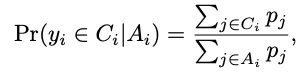
where the p‘s are the players’ true usage on the team. In real life, we never know the values of p, just as we agonizingly forced upon ourselves in the example above. Therefore, we take our sampling design (lineups) and observed usages at the player and lineup levels and perform an estimation procedure.

The likelihood function for the incomplete multinomial distribution is given by:

where p is the vector of true usages for the players of on a team, a is the observed chances executed by a player, b is the variable cell counts associated with the different lineups, and S is the matrix indicating the player lineups.

For the example above, we have

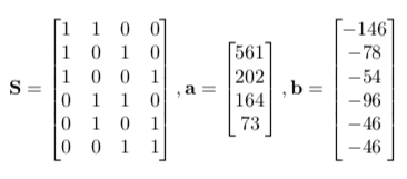
We use the designation of the count b as being negative due to the offset of chances – first player. Yes, the players are ordered in terms of most used to least used.

Attempting to solve for p is this distribution is challenging. The maximum likelihood method leads to a series of equations:

Drat, there’s that pesky sum of probabilities must be one, again. Seriously, however, we have four equations resulting from the MLE problem. Note that the (i) term indicates the row vector in S. The value, TAU, is an auxiliary vector that arises in the computation of the MLE; and therefore can be “injected” into the second equation, provided the inverse necessarily exists in the top equation.

Weaver Algorithm

As there is no analytic solution for the MLE, we can perform an optimization. A proposed algorithm by Fanghu Dong and Guosheng Yin identifies a numerical method for applying a fixed-point interation methodology for finding an optimized maximum likelihood estimator for the incomplete binomial distribution. They call this the Weaver Algorithm after the mechanical weaving machine.

</pre>
p = np.array(np.ones(4))/4.
s = np.sum(a) + np.sum(b)

error = 1
while error > .00001:
	tau = b/np.dot(delta,np.transpose(p))
	print(tau)
	temp = a/(s*np.array(np.ones(4)) - np.transpose(np.dot(np.transpose(delta),np.transpose(tau))))
	print(temp)
	pup = temp/sum(temp)
	error = np.dot((p - pup),np.transpose(p-pup))
	print(error)
	p = pup

print('True Usage: ', trueP)
print('Estimate: ', p)
print('Uses: ', a)

Using this code above, we obtain estimates of the true usages:

That is, the estimated true usages are (.587, .185, .154, .073) which are much closer to the truth; which are (.60, .20, .15, .05).

Application: 2018-19 Brooklyn Nets

For the 2018-19 NBA season, the Brooklyn Nets had a total of 19 players on roster that led to 637 different lineups of the 11,628 possible lineup combinations. Of these 637 lineups, 439 lineups managed to draw at least one chance. That is, a total of 198 lineups such as

Jared Dudley, Ed David, Shabazz Napier, Joe Harris, and Treveon Graham

played together for at least one game and registered zero chances.

Restricting ourselves to all lineups that participated in at least one chance, we find the distribution of chances executed by player:

Here, we see that D’Angelo Russell maintained the most chances for the Nets with 1860 estimated chances. Significantly behind Russell was Spencer Dinwiddie at 1137 chances. Using conditional usage, this is 31.1% for Russell and 24.2% for Dinwiddie.

At the team level, this turns out to be much smaller at the team scale. Running Weaver’s algorithm, it turns out that Russell’s overall usage is closer to 24 percent!

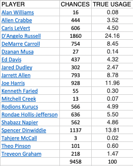
We see that Dzanan Musa’s usage gets corrected to reflect his playing time and that, despite only taking 19% of Brooklyn’s overal chances, D’Angelo Russell doesn’t tumble down towards 19%. Instead he “corrects” to 24.16%.

Using the unbalanced incomplete block design, we obtain an estimated 31.4% usage across all lineups, not far off from the measured 31.1% as before. Therefore recovery using the sampling frame is shows that Russell’s “scheduling” as a 24.16% player would indeed result in a 31% usage player.

Comparison: 2018-19 Denver Nuggets

We can compare the Nets to the Denver Nuggets. The Nuggets played with a total of 18 players during the 2018-19 season and used even far fewer lineups that resulted in chances: 329.

The Nuggets are used as a contrast only to show what a “top-heavy” team does with respect to true usage:

In this case, we see the Nuggets primarily use Jamal Murray and Nikola Jokic. This is no surprise. Their respective values of 24.9 and 27.4 come down a bit, but the relationship/offset remains relatively the same.

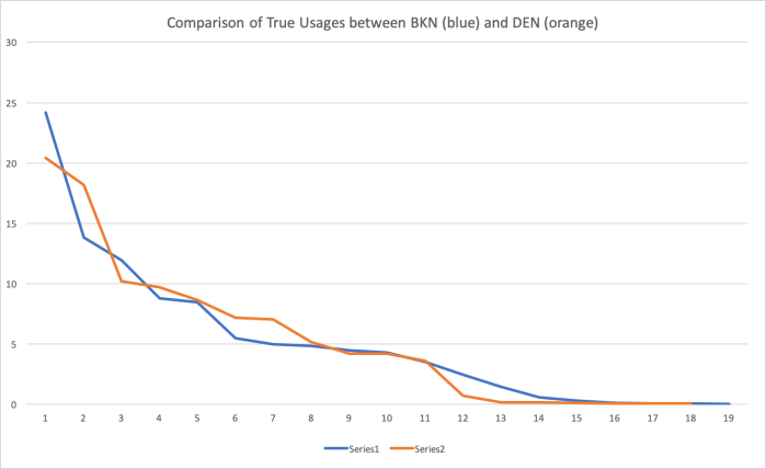
Here we see the comparison of Denver and Brooklyn as usage of players in order of highest to lowest. In this case, that despite Denver having the “star power” of Jokic and Murray, they also maintain a stable 7-man rotation; whereas Brooklyn has 5-man rotation. Typically, teams want to run with 7-8 man rotations.

Brooklyn’s knock on usage comes from the cost of injury as the team managed to have only 6 players play 65 or more game; a minimum of 80% of the season.

The takeaway here is we get to use an incomplete sampling frame to being to understand the underlying value of players within a system. A significant challenge of this algorithm, however, is the aspect of injury.

Under this model, the rotations are assumed to be at the discretion of the coach. However, a player may not play due to injury. Therefore a much more advanced model is needed to be used. That, in turn, is called the censored incomplete multinomial model. But that’s for another day.