In a recent post, we took a brief glimpse at offensive rebounding and discussed some pro’s and con’s about crashing for rebounds and provided an illustration about where rebounds go after missed attempts. In one such instance, you would have seen this plot:
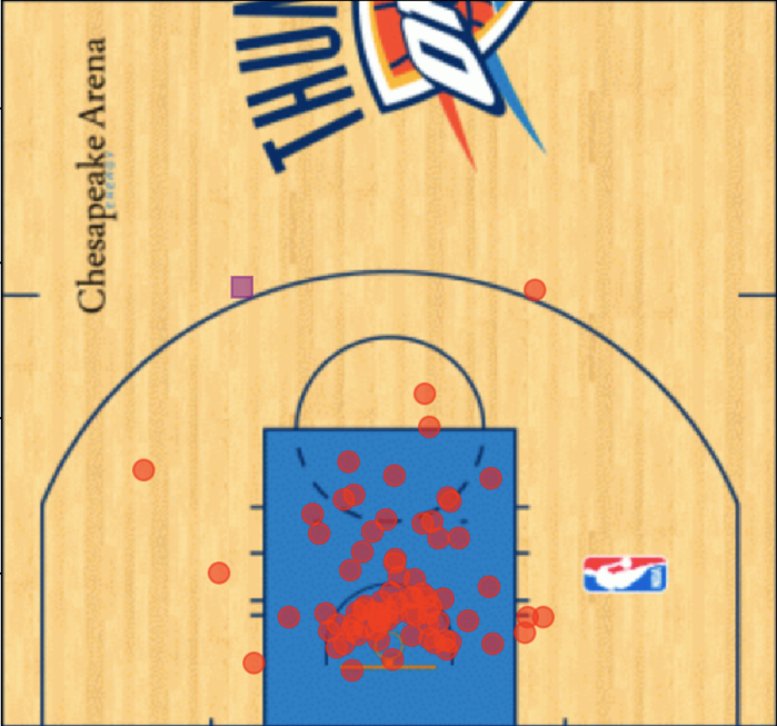
Purple Square: Location of FGA. Red Circle: Location of Rebound
For the sake of argument, let’s suppose that every single red circle in that image is an offensive rebound. Then as one chance is exterminated (through a rebound), a new chance begins in that location; extending the possession. In this case, the shot clock resets to 14 seconds and the play continues. In a post from over a year ago, we looked at where the new chances go after an offensive rebound. You would have seen this Steven Adams plot:

Distribution of FGA after a Steven Adams offensive rebound. Red Dots: Missed attempts, Green Dots: Converted Attempts
From this Steven Adams plot, you’d see that not only does an offensive rebound create a new chance for the possession, but it creates a new chance for any player on the court. This means a significant amount of second chances generated by a single player are not necessarily put-backs.
But how do we model the number of second chances on a possession? Afterall, there are only so many ways to terminate a chance: made Field Goal Attempt (no foul), made x-of-x Free Throw, Defensive Rebound, Turnover, End-of-Period*, and Offensive Rebound. There’s only one way to extend a chance. Note the asterisk on end-of-period attempts. Typically, a team rebound to the defense is tagged on heaves that would be rebounded after time has expired. Example from the 2018-19 NBA season:


Therefore, to model the amount of second chances, we can focus on chaining the probabilities of obtaining offensive rebounds together to obtain the expected number of second chances in a possession. To this end, we will start simple and then raise expectations.
Simple: Geometric Distribution
To start simple, we introduce the geometric distribution. To give an illustration, let’s consider a toy example. Suppose that you are at a court taking a series of field goal attempts; aka “shooting” at the park. At the end of the period, you decide to “leave on a make” and take a series of three point attempts until you make one to feel good about yourself leaving the court. Finally, let’s suppose you are realistically a 27% three point shooter. The question is then, how many attempts do we expect you to take until you get to leave the court (somewhat) happy?
Assuming that every shot is independent (effectively saying that the hot-hand fallacy is indeed a fallacy) and identically distributed (every three point attempt has the same probability of going in), then we have what is called the geometric distribution.
Illustrating its probabilities are simple:
Probability of Taking 1 3PA: 27%
Probability of Taking 2 3PA: (1-.27)*.27 = 19.71%
Probability of Taking 3 3PA: (1-.27)*(1-.27)*.27 = 14.39%
And so on and so forth…
The way we calculate the probabilities for the number of attempts is to multiply the probability of a miss until we hit the final attempt. Note that we always leave (somewhat) happy and therefore the final shot is the only made attempt. Therefore, the probability distribution function is given by
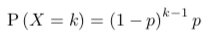
where p is the probability of making the three point attempt. Go ahead and stick in .27 for p. You will recreate the probabilities above. Here, X, is just the random variable: number of three point attempts taken. Theoretically, we could have the worst luck and take infinitely many attempts. Under this case, taking 20 such attempts would amount to .0005 (.05%) probability. Note that k in this context is the number of chances!
But how many attempts are expected? To compute this, we just compute the expected value. However, for the uninitiated, there is a bit of “sorcery” in computing this value:

Glorious math!
Using the p = .27 from above, we obtain an expected 3.70 attempts to closeout the day. So the next time it takes you approximately 2-7 attempts to close out your sessions, congratulations! You’re most likely a 27% shooter.
Application to Extending Possessions
Applying the geometric distribution to offensive rebounding produces an extra wrinkle. First, not all chances end in rebounds. Recall that offensive rebound percentage (OREB%) is computed as the number of offensive rebounds divided by the number of rebounding opportunities. Hence that 22.9% for the 2018-19 NBA season is on rebounds alone. Therefore, we need to identify the probability a rebound occurs! To this end, we look at the proportion of chances that end in rebounds.
To start, there were a total of 118,396 missed field goal attempts and 6,805 missed final free throw attempts during the 2018-19 NBA season. That accounts for 125,201 potential rebounds. Of which, a total of 25,454 were offensive rebounds and 85,653 were defensive rebounds. This leaves 14094 rebounds unaccounted for (11.45 rebounds per game). These are team rebounds. For example, the particular game mentioned above contained 20 such rebounds. Simply comparing offensive to defensive rebounds above, we obtain the 22.9% number used on Basketball-Reference.
Given the number of possible rebounds, we must also account for non-rebound situations. In this case, we have 101062 made field goals and 24803 made final attempted free throws. Note that we also must identify “Plus-1” situations, of which we had 7,419 attempts; 1788 of those missed. Note that these only take away chances!
Therefore, tallying up the numbers: Field Goals Made account for 101,062 chances. Free Throws Made account for 24,803 chances. Turnovers account for 34,644 chances. Missed Field Goals account for 118,396 chances. Missed Final Free Throws account for 6805 chances. Then we must subtract the Made “Plus-One” Events of 5631 chances. Note that this is back of the envelope math; plus-one events are including technical fouls; as the goal here is showing how the model would work.
To this end, we end up this generalized chance ending probability distribution:
- Missed Field Goal: 42.27%
- Made Field Goal: 34.07%
- Turnover: 12.37%
- Free Throw Made: 8.86%
- Free Throw Missed: 2.43%
Wow, that actually turned out to be 100% of chances. Note that we eliminated end of period chances as they have no bearing on games; as heaves are included (but insignificant) above.
From all this, the probability of extending a possession is 10.24%. This, of course, assumes the same 22.9% OREB% on free throw attempts, which (except for Steven Adams) we know is not true. Again, goal is to show how the model works.
Applying the geometric distribution above, we find that for any random possession we expect 1.114 second chances. For a game of 100 possessions, this equates to 11 second chance possessions!
Increasing Expectations: Adding in Location
For the example above, we saw that on average, we should expect a team to gather 11 second chance opportunities in a game. Unfortunately, not all teams are equal. For instance, the Chicago Bulls and Milwaukee Bucks tended to eschew offensive rebounds last season whereas the Oklahoma City Thunder tended to hunt them down. To their credit, this is due to a combination of positioning, game planning, and luck of the bounce.
However, that 22.9% is completely unrealistic. For example, a single season tends to have approximately 600 rebounds on missed FTA’s in a season. With roughly 6800 missed final free throw attempts, that’s an OREB% of 8.8%, far below the 22.9%.
Similarly, we can look at the distribution of offensive rebounds off of missed field goal attempts:
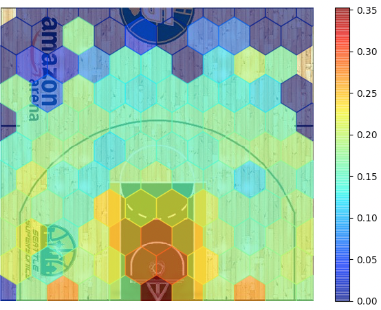
Since everyone loves hexagon plots…
Here, we see that shots at the rim push up towards 30-35% for offensive rebounds. The rate dies out dramatically at the midrange (dropping to approximately 12%) before jumping back up to 22-27% around the perimeter. There is a little flare-up of 23% at the 30 foot mark. That’s primarily Damian Lillard’s attempts and Portland reacting accordingly.
Now instead of writing everything out in terms of the geometric distribution, we start with the geometric distribution and swap out the over generalized p parameter of offensive rebounding percentage. Instead, we obtain this form of the “geometric” distribution:

Little harder, but I know you understand this!
This is the exact same form as the old geometric distribution, but instead of p we have p_{j,j+1} which is the probability of obtaining a rebound for a chance starting in state j and ending in state j+1.
For instance, let’s start with p_{0,1}. This is the initial chance. This probability would be dictated by the start of a chance: rebounded miss, turnover into transition, dead ball. A good place to start understanding the impact of initial chances can be found from Seth Partnow of the Athletic. Hence p_{0,1} in this context is the probability of terminating a possession and 1 – p_{0,1} is the probability of obtaining an offensive rebound!
Continuing on, we can look at the probability of terminating a possession after an offensive rebound. This would be p_{1,2}. Note again, that 2 here means second chance. Furthermore, p_{2,3} would indicate another second chance after 2 offensive rebounds. Again this probability would be identified by its initial position of the rebound starting a new chance (see the Steven Adams plot above for context).
Now, applying the same analysis as in the geometric distribution, we find that the Milwaukee Bucks would expect a mere 8 second chance attempts per 100 possessions while the Oklahoma City Thunder would expect 16 second chance attempts! And now we start gaining insight into the baseline model of extending possessions for any given team.
Given this set-up we can now start asking and answering questions such as “how do teams generate second chance opportunities?” and “how do teams utilize their second chances?” down to the “How are we at defending against second chance opportunities?”
For instance, limiting the Thunder to 11 second chance opportunities is a good thing. Against the Chicago Bulls, not so much.


