As a player traverses across the court, they break down and process every event that they see: the assertion of defensive players, the alignment of their teammates, and current state of the game. The ability to perceive all three components simultaneously is what I call court vision. It is one of the primary instigators that trigger the decision making process and resulting mechanical process of a player. If a ball handler registers that a backdoor cut by a teammate is being made towards the basket and ascertains that the passing lane will be open, the ball-handler may respond with a pass. At this point it is up to the player’s mechanical ability to get that pass to their teammate. The combination of the player’s decision making process and their mechanical ability is what I call a player’s basketball IQ. In other words, basketball IQ is the measurement of a players understanding of the game with respect to the physical limitations of their and the other nine players on the courts’ bodies.

The grand challenge is the ability to adequately measure a player’s basketball IQ. Instead, we focus on the components such as court vision. For, a player may have wonderful court vision but limited mechanical (compared to their counterparts) ability to score. Likewise, some players may be physical beasts and can devastate competition without understanding the value of the pass; like Wilt Chamberlain before he was encouraged to pass more and went on to lead the league in assists two seasons later. But how do we measure a player’s court vision?

One method to measure court vision is by proxy: the process of taking observable values and applying them to parts of what is agreed upon to be a sub-task of true underlying measurement of interest. We say sub-task as many proxies may be used to create an overall understanding of the quantity of interest.

For example, what makes a “great” defender? We could use a proxy of steals but not all defenders are credited with a steal even if their defense causes it. We could use a proxy of blocks but not all blocks take away possessions (only chances). We could use coverage of a player, but now we have to define that term in a way that people can agree. Or we can eschew defense and infer it from a higher level through regression methods.

For court vision, we focus on the offensive component and look at one of the proxies: passing directionality. We choose passing directionality because while it is a very simple item to understand, there is an underlying difficulty that arises when trying to say anything intelligent about it, and we have the cut locus to blame.

Passing Directionality

Passing directionality is the direction in which a player attempts a pass. For every pass a player makes, the ball exits with an angle from some reference frame.

To gain an understanding of a reference frame, consider an airplane traveling over the surface of the Earth. We care about two horizontal vectors, East and North. North points out the nose of the plane. East points out the right wing. But we also care about Up, which identifies where the ground is below us; a very important thing to know when flying. If, at any time the ground cross into North, our plane is pointed directly at the ground. Here, North is the principal vector of the reference frame and the angle towards the ground is the azimuth.

In terms of passing, since we never know the way a player is facing, we proxy their reference frame by assuming players always want to go to the basket. Therefore, the reference frame always has the principal vector facing the basket. In this case, any passes in the direction of the basket will have azimuths between -90 and 90 degrees. Any passes away from the basket will have azimuths between -180 and -90 degrees; as well as between 90 and 180 degrees.

Here, we also note that passes to the left of the player are positive angles: 0 to 180 degrees while passes to the right of the player are negative angles: -180 to 0 degrees.

Now, if we look at a pass from this player’s position, we have two vectors in the embedded space of the court. Using the embedded space of the court allows us to identify the angle from the principal vector in the reference frame. This is through the dot product:

Here, P is the reference vector, defined by the location of the basket (25,5.25) from the player (x,y). Then P = (25 – x, 5.25 – y). We similarly compute Q, the pass vector as the receiving player (x’,y’) from the player. Hence Q = (x’ – x, y’ – y).

In code, this is relatively straight-foward with start being the player and end being the receiving teammate:

Now that we have directions of passes computed, not we can start to do some analysis… Unfortunately, we just opened a big can of worms. Namely, passes are no long Euclidean. Instead, they are Spherical data of dimension one and computing something as simple as a histogram fails (gives false results).

Circular Data: Density Estimation

Using the reference frame approach, we now have a collection of angles. As the angles range from -180 to 180 degrees, we describe a circle instead of Euclidean space. The key differences are that ONE: the differences in pass direction are measured in angles not distance; and TWO: we have a cut locus. A cut locus is a place where multiple “straight lines” converge at the same point. Using key difference one, we are saying that a straight line is the arc length of the circle defining the direction of the pass. Using the reference frame above, the cut locus is at 180 degrees! This is a player making a pass directly away from the basket.

Knowing that tracking data is not quite deterministic (we can get different measurements for the same player location), we should not rely on the vectors directly, but instead focus on the probability distribution of a player’s pass direction. This amounts to computing a density estimate on the circle.

If we perform a naive analysis and apply straightforward kernel density estimator, the cut locus will give us a probability jump and throw away potentially important data. For instance, if a pass is made at 179 degrees with a reasonable error of three degrees, then we know the pass can be made between (176,180) degrees AND (-180,-178) degrees. The usual KDE will ignore the second interval and the resulting interpretation is that the pass simply “disappears.” Unfortunately, passes cannot disappear into the Upside Down.

Instead, we must perform manifold kernel density estimation to understand the distribution of passing direction.

Circular KDE

The usual kernel density estimator is given by

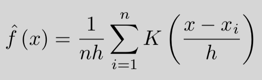
where n is the sample size, h is the bandwidth, and K is the kernel smoothing function. For a given player, we can look at a collection of n passes of interest. Each pass is then viewed as a noisy estimate with some measurement error (bandwidth). The resulting kernel function is how that measurement noise is distributed about the measurement.

In classical kernel density estimation, the most common kernel function is the Gaussian smoother:

So we must use an analog version of this with the circle in mind. To this end, we can leverage the von-Mises distribution:

which only runs over the angles between -180 and 180 degrees. Here, mu is the mean direction and kappa is the concentration. Think of concentration as the inverse of variance. The larger kappa is, the tighter the distribution is about the mean. However, thanks to the cyclic nature of the cosine function, we ensure that passes don’t disappear when it crosses the cut locus.

The sacrifice we make is that the bandwidth is no longer separable. Under the von-Mises distribution, the bandwidth is absorbed into kappa and is contained within the modified Bessel function of kind zero defined by

which ever-so-nicely ensures that our probability distribution integrates to one!

Using this set-up, our circular kernel density estimator is given by

where now a larger bandwidth indicates the same things as a small bandwidth in the traditional kernel density estimation methodology.

Application: Steven Adams

As an application test case, let’s look at a subsample of passes from Steven Adams of the Oklahoma City Thunder. Here, we take the position of Adams at every pass, calculate the angle between the pass and the basket at Adams’ position, and mark that as an orange dot. Using zero degrees as the reference frame’s principal vector, we draw the circular manifold in green and apply the kernel density estimator above:

Here we see that Adams primarily makes passes to his front left at approximately 45 degrees and to his right front at approximately 40 degrees (320 degrees on the plot). Here, the green circle represents the manifold which describes the passing direction. Zero degrees always points to the basket. The blue line is the kernel density estimator. This shows that Adams primarily attacks the rim with his passes, but tends to favor his left.

At the high level, this is informative, however, we have lost the court information. We don’t know where Adams is making passes. More importantly, we don’t know if his passes are location dependent. For example, does Adams pass different from the left elbow than the right elbow?

To understand this, we must perform a conditional distribution.

Conditional Kernel Density Estimation: John Wall

When we condition the circular kernel density estimate, we begin to see the dependence of the passing directions based on the player position. Steven Adams is not a great example to show this off. Instead let’s take a look at John Wall.

At the left of the top of the arc, we find that Wall primarily passes towards the corner. Note that this doesn’t suggest passes do go to the corner. Only the direction. This can be passes leading into a give-and-go with a post player as well. However, we see that at this location, his passes tend to go left and forward at about 80 degrees.

However, if Wall move in to the foul line, we see the distribution of his passing change to looking in two directions with a slight preference to the right. At a cursory glance, this my be a reaction to a weak-side defender stepping up to cut potential drives. From the angular point of view, this is most likely a “kick” pass to the weak-side three point line as the direction points to below the break.

If Wall gets into the lane, we see that his passing almost goes entirely to the right. The small pocket to the left is pointing towards the dunker position, which is most likely a dump pass to get the ball out of congestion. The blip right to the rim is an oop passing lane. However, predominantly (over 75% of the time) the pass is getting kicked out.

Let’s put this all together and simulate a drive by Wall.

Here we see how the “court vision” with respect to passing plays out through the course of a drive. We can now start to perform other methods of analysis to better understand changes in passing vision; such as “do weak side defenders help?” or “If I position a defender in this location…” We can partition the distributions and perform circular distributional tests.

For the remainder of the article, let’s enjoy the subtle differences of players…

Malcolm Brogdon: Indiana Pacers

While Brogdon is on the Pacers for the 2019-20 season, his data was collected for the 2018-19 season with the Milwaukee Bucks. Here, we see a very Milwaukee-centric style of play.

As he traverses the same path as Wall, the passing vectors go backwards towards most likely Giannis Antetokounmpo and Brook Lopez. But as Brogdon attacks the rim, his passing directions change to the dump pass to the strong side block and out back to the right wing on the weak side. This was a Bucks’ staple in exposing the weak side collapse for open looks a the perimeter.

This type of passing regimen comes from a distributor who is not a primary option on scoring, but rather a player that protects the ball and forces the defense to swarm. These players tend to look away from the basket and create mid-range and beyond-arc opportunities.

Jaylen Brown: Boston Celtics

Jaylen Brown follows a similar pattern to Brogdon with one slight difference: A high-low passing vector emerges during the drive. Boston, notorious for off-ball players beating their defenders baseline, shows that Brown looks for that pass during the drive.

Also notice the the zero vector is almost pinched to absolutely no distributional weight. This is very apparent when Brown gets deep into the lane. This indicates that Brown is not passing to score. He is going for the layup. In Brogdon’s case, he is still looking for a dump underneath the hoop, or a dunk from a teammate. In Brown’s case, he’s attacking the rim himself.

The left and right bulges in the distribution within the key are dumps and kick-outs. He tends to look for “at-the-break” players and anyone near the strong-side block. This is the profile of an attacking guard within a system.

LeBron James: Los Angeles Lakers

Looking at one of the biggest names in the game, LeBron James is yet another style of player. James fits the profile of an attacking guard but without a system.

James starts with the standard perimeter passing profile at the top of the key, but as he drives into the lane, he predominantly looks short corner strong side and below-the-break weak side. Once he gets into the lane, he becomes one of the most dangerous players in the league: uniform attacker.

This type of distribution shows that all the weight goes just forward. There is a slight bulge towards the strong block, but weak elbow, weak below-the-break, and anywhere near the rim becomes primary options. This suggests that James reads and reacts to the defense accordingly.

One he gets deep into the lane, there’s three passing options: strong-side dunker dump, kick-out to weak side, and alley-oop to the strong side rim. There is no wonder why James averages 8-9 assists per game despite being a premier scorer and playing usual starter minutes (~35 a game).

Steph Curry: Golden State Warriors

Steph Curry follows the same form as LeBron James when it comes to attacking the rim. Curry keeps a large distribution in front of him, as opposed to peaking in certain directions.

That is, until he gets into the lane. At this point, he beings to look weak-side block. It is this position that players such as Klay Thompson are cutting behind the defense (Boston-esque in that nature) or players like Andre Iguodala and Shaun Livingston were waiting for the defense to collapse to get potentially open looks at 3-10 feet from the rim.

Compare to Wall above, who almost completely turns into a right-only vision player; we begin to see why Golden State is more likely to beat you from anywhere rather than the Washington Wizards: half the court disappears on drives in Wall’s case.

Next Steps

Armed with some simple manifold nonparametric learning as circular kernel density estimation, we can begin to understand some of the vision associated with players. Merely one small piece of the pie in decision making.

However, we are able to start performing testing of certain player capabilities or schemes. We are also able to “scout” player tendencies, and more importantly: quantify them.

And even more so importantly, we are able to start attaching probabilities to actions. Instead of quantifying passes by proxies through “win probability” or “change in shot quality,” we can now quantify the probability of a pass as “how likely will he actually make this pass?” At the scouting level, it tells me where I can make an adjustment.

Plus, the animations are a little cool, too… right?