Back in 2013, Wired put forth an article detailing an effort by Dustin Cable at the University of Virginia’s Weldon Cooper Center about mapping a point distribution of races in the United States. The map is constructed from the 2010 United States Census and places a color coded dot for each of the geolocated (by address) 308,745,528 persons identified. The color codes work as follows: blue dots represent white Americans, green dots represent African-Americans, red dots represent Asian-Americans, orange dots represent Latino-Americans, and brown dots represent the remaining races. The result is an amazing 7 gigabyte visualization identifying the diversity in the continental United States.
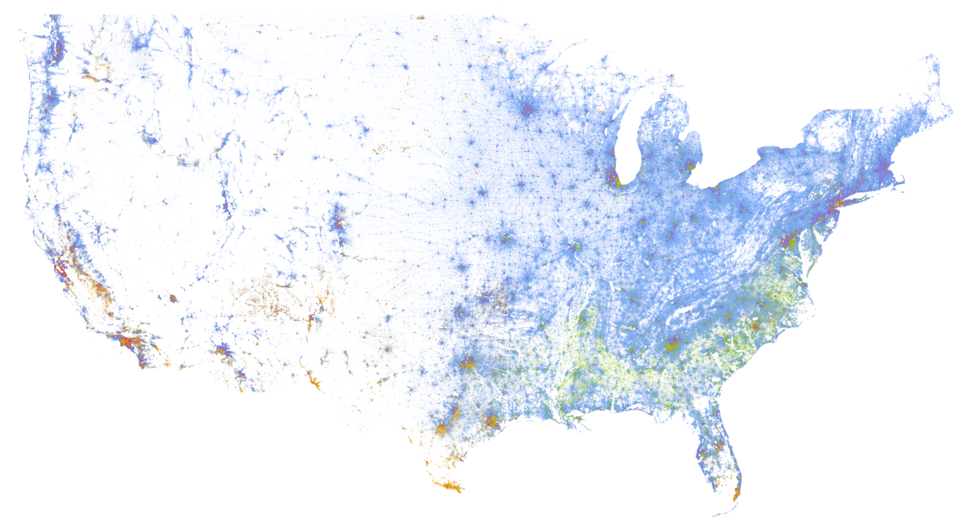
Distribution of Races in the United States, derived from the 2010 United States Census. Visualization provided by the UVA Weldon Cooper Center for Public Service.
Using this map, we can zoom in and take a look at each major city and their distribution of races. For instance, let us consider Baltimore, Maryland. Baltimore had a 2010 population of 620,961 persons with an approximated 391,826 African-Americans;175,111 white Americans; 29,185 Latino-Americans; 16,766 Asian-Americans; and 8,073 of other races.
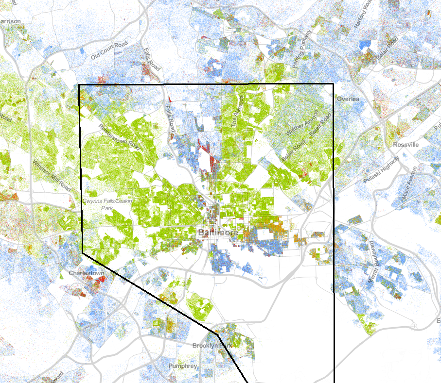
Distribution of races in Baltimore, Maryland according to the 2010 U.S. Census. (Blue = White Americans; Green = African Americans; Red = Asian Americans; Orange = Latino Americans)
From the Baltimore map, we see that there are is some separation between races between neighborhoods. However, the Johns Hopkins area of Baltimore (North Central) looks quite integrated. Similarly, the areas around the Inner Harbor region appear to be well-integrated. Despite this, Western Baltimore has a fairly uniform African-American distribution in population. The question is then: “How integrated is Baltimore City?”
We can construct simple measures (and will later), but we must define some constraints for our measurement. For instance do we call a uniform population not integrated? In Baltimore, we may say yes. But what about cities such as Oregon, Wisconsin?
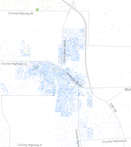
Distribution of races in Oregon, Wisconsin; according to the 2010 U.S. Census.
Oregon, Wisconsin had a total population of 9,231 persons with approximately 8,686 White-Americans; 203 Latino-Americans; 111 African-Americans; 74 Asian-Americans; and 157 from other races. Looking at the map, the city is primarily white, so should the integration method identify this village is poorly integrated or well integrated in the absence of other races? It should be noted that the square patch of primarily African-American population off County Road M is the Oregon Correctional Center.
Construction of a Measure Relative to Population Distribution
The method of integration we will investigate will be a simple method defined off of confusion matrices. A confusion matrix is a machine learning error matrix (contingency table) that displays the truth value as a row and the predicted value as a column. A simple machine learning algorithm to use is a k-Nearest Neighbors method that counts the k nearest neighbors to a particular point and says that the person should be, in our problem, the same race as the majority of the neighbors. The rows of the confusion matrix are the races of each individual person, and the columns would be which race that person should be. In our problem set up, we have five rows and five columns: White, African, Asian, Latino, Other.
Let’ consider a basic example. Let’s suppose we only care about the nearest five neighbors within a village of 50 people. In this case, let’s assume that each race has the exact same count: 10 persons each for each race. If the five categories of races are not integrated at all, then we expect a diagonal matrix that will have 10’s down the diagonal. If the categories of races are well-integrated, then we expect 2’s in every entry. This would be a uniform distribution across all race categories, indicating a well-integrated distribution of population.
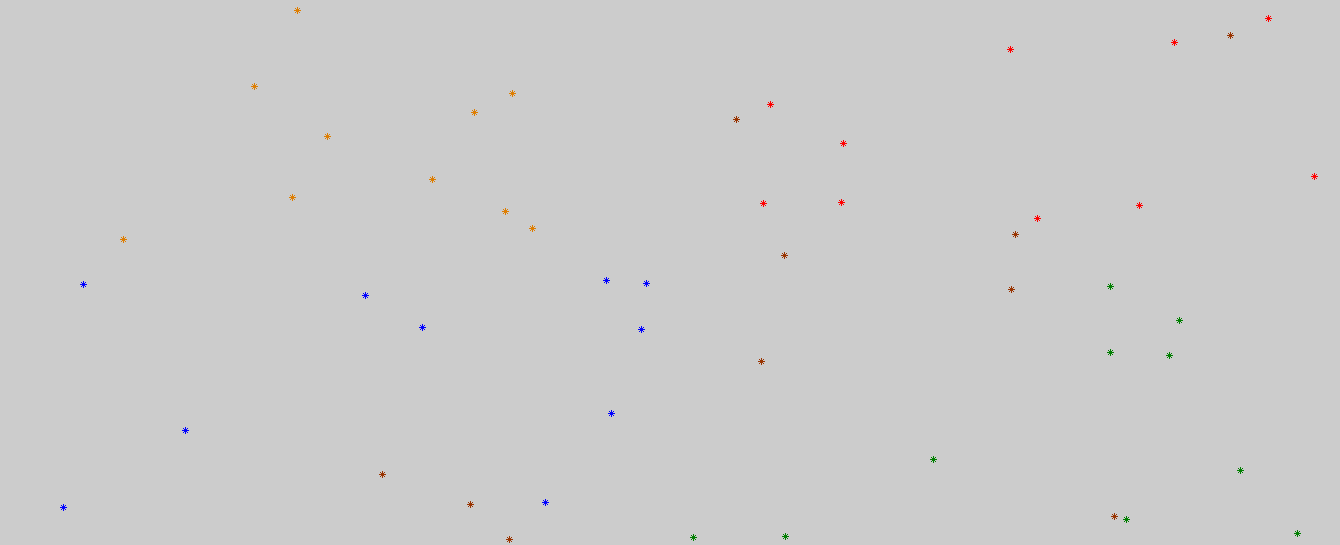
Simulated distribution of a poorly integrated neighborhood.
Considering a poorly mixed distribution simulated in this example, we consider the orange dots (Latino population) in the upper left corner of the distribution. Selecting a nearest neighbor of 5 persons, we count the number of each race category and select the one with the highest count. In the case of a tie, we select the next point outside of the neighborhood to serve as a tie breaker (instead of random selection). For this example, we get the following k-Nearest neighbor labels: O, O, O, O, O, O, O, O, Bl, Bl. That is, eight of the Latino persons live in a ‘Latino neighborhood’ while two Latino persons live in a ‘White neighborhood.’ The corresponding row in the confusion matrix is (2,0,0,8,0) for (White, African, Asian, Latino, Other) categories. Completing this for all fifty points, we obtain a confusion matrix that is close to being diagonal.
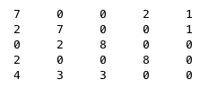
Confusion Matrix for the simulated example of 50 persons; ten from each race category. Four categories are intentionally partitioned; one is intentionally integrated.
We can immediately see the four races that are intentionally segregated and the one race category that is intentionally integrated into the other four regions. As expected, the segregated races have large values on the confusion matrix’s diagonal. The race category that is intentionally integrated looks more uniform across its row, with no large diagonal element. In this case, the diagonal element for the ‘Other’ category is zero only due to the small sampling.
Determining a Neighborhood Separation Value
We selected the value five off the cuff only because it was simple. Typically, we select a value that best separates the categories. Since we are not attempting to induce a separation on the race categories, we can select a value of k based on population density and select a distance to measure. That is, consider the number of blocks that would define a neighborhood and use the number of neighbors based on that city’s density. For example, if there are approximately 25 persons per square block, then we select a 25 person neighborhood. Typically civic engineers select 100,000 square feet per city block. For Baltimore, there are 7,671.5 persons per square mile; or per 27,878,400 square feet. This means we would select, based on a 1-block neighborhood, we would take a 27 person neighborhood.
Analyzing the Confusion Matrix
The confusion matrix will have a sum total of the population of the city. If we add up all of the entries in our confusion matrix example, we get 50. The population total. Now, we can apply a Chi-Square test to test the relationship between the actual persons and their nearest neighbors. If these neighborhoods are well mixed, then the value of the test should be close to zero. If the distributions are segregated, we expect the distributions to be big along the diagonal of the confusion matrix and therefore the chi-square test will be large.
Using our example, let’s carry out the Chi-Square test. First, we compute the expected values for each bin. This is the row total times the column total divided by the grand total. For the white population, we have 10 white-Americans and 15 predicted white-Americans. With a grand total of 50 persons, the expected value of white people in ‘white neighborhoods’ is then 15*10/50 = 3. Continuing in this manner, we get the following expected confusion matrix based on the neighborhood method.
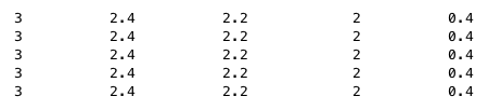
Expected Confusion Matrix based on the simulation example.
Then we take the difference between the observed and expected values and square them. Normalizing against the expected value allows us to standardize the difference between the observed and expected values. Let’s put this into plain speak. We observed 7 white Americans in a predicted white-American neighborhood. We expected 3.0 is there was no neighborhood relationship. The difference is then 4. Squaring this, we get 16; and dividing by the expected 3.0 value, we get 5.3333. Thus the index of difference segregation index for ‘white-neighborhoods’ is 5.333.
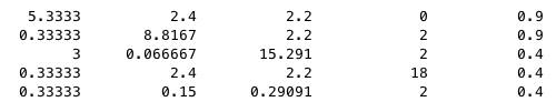
Segregation Matrix illustrating the Chi-Square values for each neighborhood. Rows are Observed Persons in each race category. Columns are the nearest neighborhood race categories.
Here, we see that the Latino neighborhood is the most segregated. Viewing the image, we definitely see this . This method now gives us an idea of how segregated the neighborhoods are. Now to compare cities, we then look at the overall sum. Adding all the entries together, our simulated example gives a segregation index of 72.348. This value has 16 degrees of freedom for every city; therefore we can compare the indices between cities. If we’d like to normalize further, we can divide by the city population to get a relative score to population index. Thus, the segregation index for our example is 72.348 / 50 = 1.44696. If the communities are well-mixed, this value will be zero. The maximum value for this is index is 20.
Application to Real Cities
If we perform this analysis for Baltimore, we have a segregation index of 1.1637. This indicates that the city is somewhat segregated, but it is nothing compared to the major three cities that top the segregation index. Here, applying this methodology, we obtained values for Detroit (17.2794), Milwaukee (16.3849), and Chicago (15.9348). This analysis was only applied to the 40 largest cities, according to the Census Bureau. Taking a look at each of these cities, we see the similar segregations found in the simulated example.
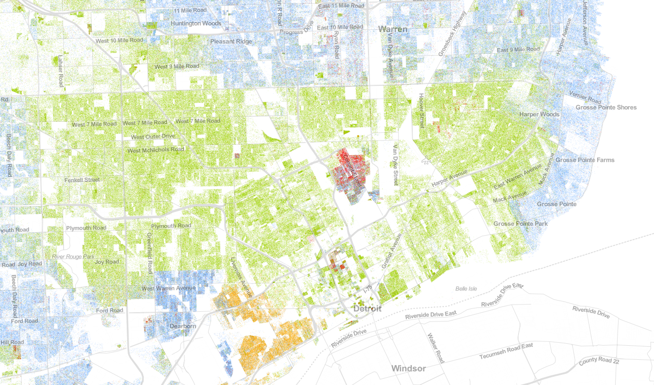
Population map for Detroit, Michigan; based on 2010 Census Bureau data. Obtained from UVA’s Weldon Cooper Center for Public Policy.
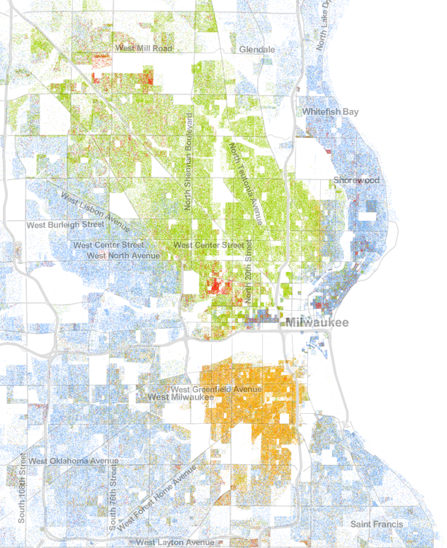
Population map for Milwaukee, Wisconsin; based on 2010 Census Bureau data. Obtained from UVA’s Weldon Cooper Center for Public Policy.
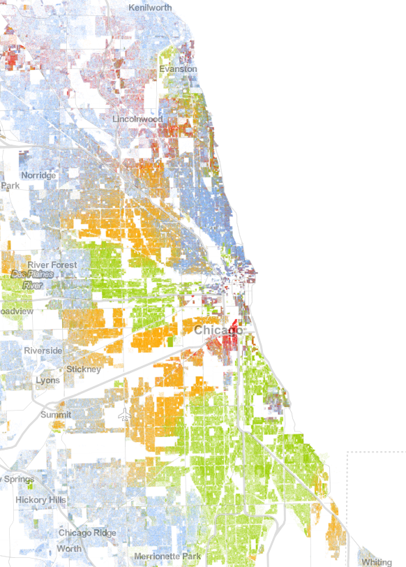
Population map for Chicago, Illinois; based on 2010 Census Bureau data. Obtained from UVA’s Weldon Cooper Center for Public Policy.
However, we also find some decently integrated cities. In fact, two of the five lowest segregation indexes come from the Triangle in Texas: Dallas (7.2383) and Houston (7.3803). However, Los Angeles ranks low on segregation (8.3494). However, the San Francisco, Oakland, and San Jose region bottoms the segregation index (5.9348).
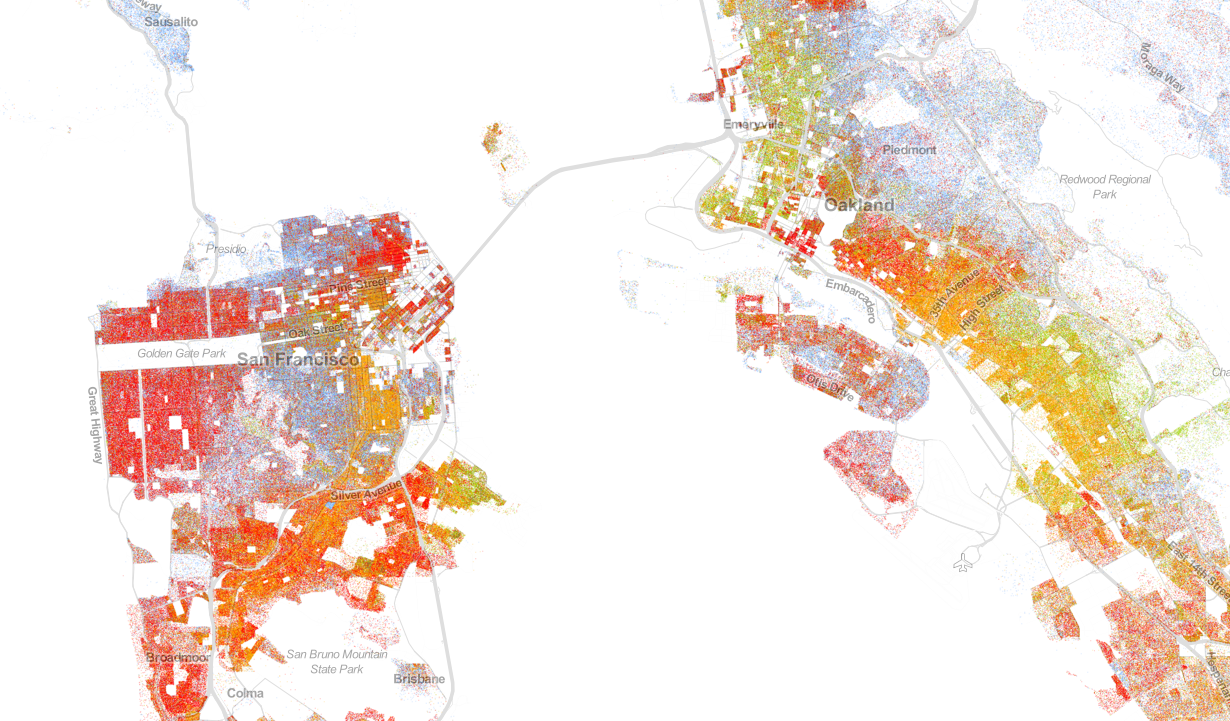
Population map for San Francisco and Oakland, California; based on 2010 Census Bureau data. Obtained from UVA’s Weldon Cooper Center for Public Policy.
As we see, this is merely a simple segregation index calculator. While there have been claims that segregation has been greatly reduced, we see it has not been eliminated. This is just a simple example to show how some cities are segregated and a simple method for calculating segregation.
*Edit: Numbers originally erroneously pinned from entry (1,1) of confusion matrices. Updated to reflect total index.

Pingback: Oakland, California | Squared Statistics: Analyzing Crime, Sports, and People