In a recent post, we identified the Colley Matrix methodology for ranking NBA teams. The methodology provided insight but abused the originating statistical construct in an effort to enforce a correlated, solvable, set of equations to identify a “probability” of winning. Unfortunately, we witnessed that not only were those statistical assumptions violated, but the resulting probabilities could be over 100% or negative. In this article, we focus on a probabilistic framework for measuring pairwise comparisons of teams through the use of home-away indicators and win-loss results.
The most common model of this type is the Bradley-Terry model.
Bradley-Terry Model
The basic form of the Bradley-Terry model focuses on pairwise match-ups between teams, dependent on location, and records whether the home team has come away with a victory. To model this, the explanatory matrix, X, is an N-by-31 matrix of variables, where each row of the matrix represents a game. We use 31 variables to identify the 30 NBA teams, as well as an intercept term to correct for global mean of the observed results.
Each Row is a Game
With the idea that each row of the explanatory matrix is a game, we indicate the home team as a “+1” and the away team as a “-1” value. For the intercept, we set the last value in the row to “+1.” For instance, last night the Boston Celtics defeated the Los Angeles Lakers 107 – 96 in Los Angeles, CA. If we place each team in alphabetical order, the Celtics are the second entry in the row, after the Atlanta Hawks, while the Lakers are the 14th entry in the row, after the Los Angeles Clippers. This means that the second entry in the row is “-1” as the Celtics are the visiting team and that the 14th entry is “1” as the Lakers are the home team. The final entry is the value one to correct for the intercept.
This means that the row of the explanatory matrix is given by
(0,-1,0,0,0,0,0,0,0,0,0,0,0,1,0,0,0,0,0,0,0,0,0,0,0,0,0,0,0,0,1)
Regression Would Be Nice…
Now, if we are able to write the result of the game in terms of a random variable conditioned on the teams playing and location played, a common question to ask is whether we can fit the response to a linear model. Why linear? Consider this fit:

Here, Y_i, is the response for Game i. This can be whatever the response we feel is right. Want to use the result of the game? Want “+1” for home win, “-1” for road win? Sure, go ahead. However, we must be careful of the resulting distributional properties after we make our decision. For instance, using least squares will not work properly if we use “1” and “-1.”
The beta values are the weight given to each explanatory variable in predicting, or explaining, the response. In the Bradley-Terry Model set-up, let’s apply the Celtics-Lakers match-up:

This means the linear model compares the Lakers and Celtics by looking at their coefficients. If the Celtics are the better team, then their coefficient will be larger than the Lakers’ coefficient; provided the larger the response, the more likely a team wins the game.
Using the explanatory matrix notation above, we immediately see that beta_0 is the league-average home-court advantage.
The epsilon term is simply the additive error in the model. This means that while two teams play each other, and one is favored, there is some sort of associated error that could have us seeing a response that is not likely. Accounting for resulting situations like when the Sacramento Kings defeated the Oklahoma City Thunder on November 7th.
This given model is not quite correct, because the response is not well understood. Persisting with usual least-squares will lead us to predicting real values instead of win-loss; which is what we are ultimately after.
To account for this, enter logisitc regression.
Logistic Regression
Logisitic Regression is a methodology for identifying a regression model for binary response data. If you are familiar with linear regression, then the following explanation can be skipped down to applications to NBA data. If you are unfamiliar, strap in, it’s going to be a mathematical ride.
Bernoulli Distribution
The Bradley Terry model makes an assumption that each game played is an independent Bernoulli trial. This means that it’s a coin flip, where the coin is weighted by a function of the teams playing and where they are playing. The distribution function is no different than that of Colley’s initial independent model without using the beta prior distribution. The Bernoulli distribution is given by

Here, p is the probability that the home team will win the game. The value, x, is actually the response. Not to be confused with the values of X above. The response is either a 1 if the home team wins or 0 if the home team loses.
Exponential Family Model
The Bernoulli distribution falls under a class of models called the exponential family model. In regression, if we are able to write the distribution of a model in an exponential family format, we are able to identify a link function that allows us to build a linear model to understand the relationship between the explanatory variables and the response. The exponential family format is given by

The value h(x) turns out to be the marginal probability measure. This is not entirely necessary for our purposes. The value, T(x), is called the sufficient statistic. This identifies a compacted way to collapse (or aggregate) the data in a manner that the distribution associated with the parameter space is unchanged. In simple terms, this is a data reduction statistic.
The value theta is called the natural parameter. This value identifies the link between a linear model and the parameter space identified by the sufficient statistic. The value, A(theta), is the moment generating function associated with the distribution. If we were to take this function and compute derivatives, we will obtain the moments of the associated distribution.
Bernoulli as an Exponential Family
Let’s start by showing the Bernoulli distribution is indeed an exponential family model.
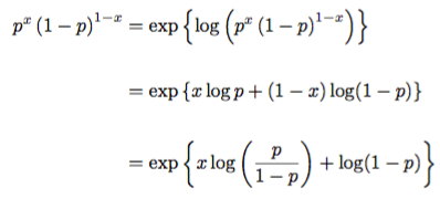
We find that h(x) =1, T(x) = x, theta = log(p / (1-p)), and A(theta) = -log(1-p). The sufficient statistic shows that the data point itself contains all information about the parameter p.
This shows that the link is the natural log of the ratio of probability of success divided by the probability of failure for the home team. Think of this as the log of the odds ratio for a home team winning a game.
Aside: Differentiation Yields Moments
While we are here, let’s verify that the moment generating function indeed yields moments. The term –log(1-p) is not in terms of the natural parameter. So let’s first find that. We start with understanding what the natural parameter looks like:

We then substitute this in to the moment generating function to obtain a function of the natural parameter:
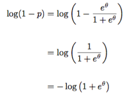
We needed that negative! Look at the exponential family model and notice that there is a negative lurking there. Here, we obtain it explicitly from rewriting the moment generating function in terms of the natural parameter! Now, let’s take the derivative with respect to the natural parameter.
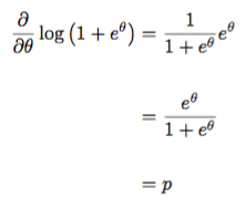
We can check the second derivative as well:

So we are indeed in business as these are the first moment and second central moment (variance) of the Bernoulli distribution!
Link Function
Now that we have an exponential family distribution with identity sufficient statistic, we can apply the link function. This is merely setting the response of the linear model above to being the link function. Explicitly, we have that

Note that since the probability of the home team winning the game is between 0 and 1, we have that the odds ratio is between 0 and infinity. Taking the natural logarithm, we obtain a value between negative infinity and positive infinity. We are in great shape for regression!
However, since we do not know p, we cannot just solve these equations for the number of games we have for the season. Instead, we look back at our exponential family for help. This process is called performing a logistic regression. The link function above, connecting p to theta, is called the logistic link.
Regression Time!
To perform the logistic regression, we do exactly as we do in standard least squares regression. We look at “squared error distance” between the model and the results and minimize these errors. In linear regression, we assume the Gaussian distribution. When placed into the exponential family model, we get squared error loss. That’s not explicitly the case here.
Let’s look at how we do this in the Gaussian case. In the basic linear regression problem, we assume homogeneity. This means that the variances are constant and fixed. We still have to estimate them, but they are viewed as constants.
The negative log-likelihood of the exponential family identifies our loss function. In this case, for Gaussian distributions, we obtain

Viola! We have least-squares sitting in front of us. To recount, the first arrow simply applies negative logarithms to the exponential family distribution for the Gaussian. The second arrow just dusts off the constant terms that have no effect on the minimization procedure.
I will leave it to the reader to verify the exponential family form of the Gaussian, which results in the identity link, theta = mu. For now, let’s do the exact same thing here for the Bernoulli distribution.
Negative Log-Likelihood
Taking the negative log-likelihood for the Bernoulli distribution, we obtain
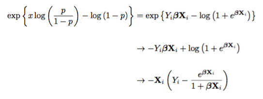
In the Gaussian case we simply take the derivative, set it equal to zero, and solve. In the Bernoulli case, we took the liberty of taking the derivative; which is the second arrow above. Setting this equal to zero and solving does not work. Thanks, Logistic function…
Newton’s Method
Therefore, an iterative scheme must be adopted. The simplest one out there is Newton’s Method. Newton’s method is a calculus based method that uses tangent lines to iteratively solve for a root (zero value). This inherently requires the functions we are maximizing to have nice tangent (derivative) behavior. To compute Newton’s method, we take the function in question with a good starting point and compute the tangent line at the function evaluated at the good starting point. Where this tangent line intersects the x-axis gives us an update for where the zero most likely is.
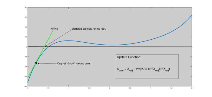
Illustration of Newton’s method. Notice if the starting point is somewhere to the right, it will run away from the actual root.
Since our function we are attempting to solve the root for is the derivative, we need to take the second derivative of the negative log-likelihood function:
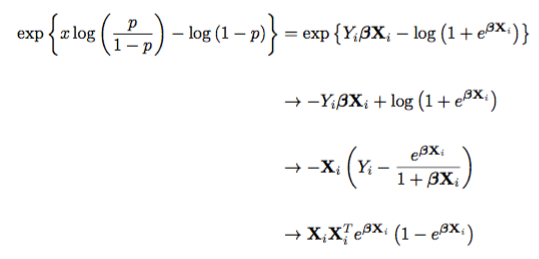
The final line is the Hessian value. Piecing this together, we obtain Newton’s method for solving for the coefficients of Logistic Regression!

After choosing a good starting point, we run this until a desired convergence. The output is the beta vector of weights for each team. The larger the weight, the higher associated probability that team has of winning.
Application to Boston Celtics at Los Angeles Lakers
With the Celtics playing at the Lakers on November 8th, we can look at all games up until November 7th and compute the Logistic Regression using the Bradley-Terry formulation. In this case, we obtain the following rankings:
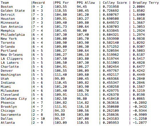
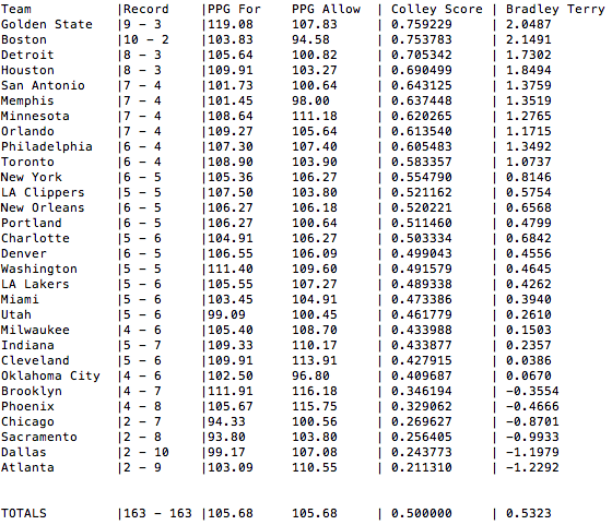
NBA standings, Points-per-Game (For and Against), Colley Score, and Bradley-Terry Rankings
Here, we find that the Boston Celtics’ coefficient is 2.0004 while the Los Angeles Lakers coefficient is 0.4828. Not shown above is the intercept; which is 0.2229. Piecing this together, we take note that the Celtics are the visiting team. Therefore the linear model is given by 0.2229 – 2.0004 + 0.4828 = -1.2947. Placing this into the logistic link function, we obtain a Los Angeles Lakers probability of winning this game to be 21.5058%.
Understanding Assumptions
Here, we must make a note that in certain cases, we obtain outrageously unrealistic cases. Let’s take for instance a proposed game between the Boston Celtics and the Atlanta Hawks in Boston. Using the coefficients above, we have that the natural parameter response is expected be 0.2229 + 2.0004 + 1.2877 = 3.5110. This leads to a Boston Celtics probability of winning this game to be 97.10%.
While the Celtics are expected to win, why is this absurd probability so high? This is in part due to large variation associated with the model. The Bradley-Terry model imposes an iterative reweighted least squares model where the weights are the associated Bernoulli variances for each game. This is identified immediately by placing the above gradient equation in terms of matrices.
From this construction, we obtain a method for approximating the error associated with the estimation of each teams’ weight, beta_j. In this case, we obtain a variance for each team to be roughly 11,200,00,000,000,000. This is the exact same problem we run into with Adjusted Plus-Minus!!!!
This shows that while we identify a ranking, despite being statistically correct, the associated variance effectively says that the ranking is simply just that; a numerical ranking. Furthermore, this suggests, through Wald type testing, all teams are equal.
Why did this variance inflation happen? First off, all teams have not played each other. This identifies that the support for the model is missing observations. When this occurs, the model is only fit for games that have at least one sample. if a game has not been seen, the explanatory matrix enforces that the win-loss response does leverage information between the capabilities of those two teams. Information lost due to the absence of observable information.
Second, the model assumes we have enough responses for each match-up in order to estimate the variance. One observation? Variance is “zero” in the estimable sense. In the model sense, this is effectively infinity as no information of variability exists.
The explanatory matrix is effectively a schedule matrix. Therefore, for each match-up, we need to see multiple observations in order to adequately estimate variation of results within that schedule.
Correcting Issues?
One way to correct for issues is to do the exact same methodology as in adjusted plus-minus. That is, apply a regularizer. This will control variance inflation, but also perform a singular value decomposition type construction, effectively muting a team’s weight. This in turn turns the team into a baseline for other teams to compare against.
In this case, we will be able to gain stable estimates, but at the cost of interpretation. In the model above, the value e^beta is the odds ratio for a team’s chances of winning. In the regularized setting, this is no longer the case.
Another way to correct is to play around with features. Try to use something other than schedule to build a Bradley-Terry model. Many folks over the years have attempted this. However, when going down this path, keep in mind the signal-to-noise problem that reared its ugly head above.
Finally Some Code
Finally, we leave you with some basic Python code to reproduce the results above.
Processing Data
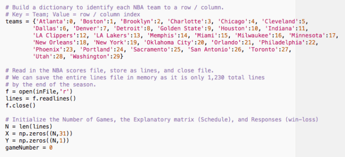
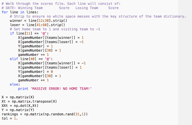
First, we process the data. Assume files where each line is date, winner, score, loser, score. Then we simply open the file, read the lines and hold them in memory. Similarly, we create an NBA team dictionary to use to indexing and identify the numebr of games played.
Populating Matrices
Next, we populate the explanatory matrix and response matrix. This is just a simple sweep through the data file. We also perform some of the basic linear algebra functions that will be needed later; such as a matrix transpose, some multiplication, and rankings initialization.
Performing Newton’s Method
Next, we perform Newton’s method to identify a set of coefficients that in turn give us our team rankings.
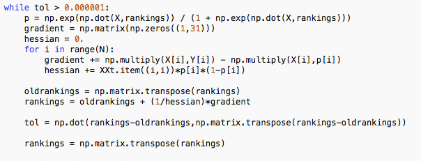
The resulting rankings vector yields our team rankings. We can simply return this as a function for a later block or display accordingly.
Also note as this is an 31-dimensional walk with a random initial start, each time we run Newton’s method, we will get different (but effectively the same) results. To tighten this component, we either have to find an optimal hot start location; or utilize a different convergence metric.
Application to Today!
As of the morning of November 9th, 2017, there has been a total of 163 NBA games played. Applying Bradley-Terry to these games, we obtain the current rankings:
How would you build your own model?
Pingback: Weekly Sports Analytics News Roundup - November 14th, 2017 - StatSheetStuffer
Hi, Justin, I was modelling Bradley Terry Model in Excel and now I find this article and tried to reproduce. The results was so good, the model is the best that I found. Thanks.
Now, I have a doubt, How can I adjust the Home Field Advantage in this model if I want analyze different leagues with different Home Fields Advantages? Maybe this is something easy to do, but I’m relatively new in programing and searching to learn more about. Thanks for the attention.
LikeLike
You’re an absolute legend for this one. Read through Statistical Sports Models in Excel but it was light on the math, and I hate excel.
LikeLike