Warning: This is a lecture from one of previous statistics courses taught over the years. It will be theoretically heavy, but offers insight on some of the research process required for developing analytics. (End Disclaimer)

 

Thought Exercise: Perimeter Defense

Whenever we develop an analytic to help describe the game, we typically have to ask three things. First, “is our analytic representative of the actual thing we are attempting to analyze?” Second, “does the analytic yield intelligence?” Finally, “is our analytic stable?” While these seem like obvious requirements, it may come as a surprise that many folks actually miss the mark on one of the three requirements of developing an analytic.

Take for instance, perimeter defense metrics. While it has been long known that defensive three point percentages do not truly reflect a team’s perimeter defense; yes that’s three links representing effectively the same view… many folks (including some pro teams!!) still use defensive three point percentage as a barometer for defining how well their team plays perimeter defense. While many will attempt to argue that defensive three point percentage does indeed measure perimeter defensive capability, it has been shown repeatedly (over at least a five season span now) that it is indeed not stable; nor does it yield actionable intelligence.

In response to fighting with survivor bias that comes from play-by-play, savvier teams, have focused on frequency and efficiency relationships; attempting to understand the “negative space” of perimeter defense. That is, of deterrence of high quality attempts and promotion of low quality attempts. Others attempt to mitigate the survivor bias by introducing “luck adjustments.” Whichever direction we choose to go for our analysis, the challenging part remaining is to determine the robustness of our measure.

In this article, we focus on defining a core statistical concept in analytics: consistency. For a given analytic, consistency identifies the “biasedness” of an estimator relative to its sample size. As the sample increases, we should expect the estimator to converge to its true value; hopefully the parameter. Consistency is a probabilistic argument that is defined by

for a true parameter, theta, and its estimator, theta_n, for some sample size n. Thus, the goal of analyst is then to determine if this equation is satisfied and then identify convergence rates of the statistic they had just generated.

Consistency: Coin Flipping Example to Be Used Later

Let’s start with a simple exercise to demonstrate consistency. Let’s consider an independent, identically distributed (IID) Bernoulli process with some probability of success, p. The most basic example is the “coin flipping problem.” So let’s start there. Suppose a coin has a probability, p, of coming up heads. Suppose we flip this coin n times and count the number of heads on the coin. Our goal to estimate the true value of p and then determine how consistent that estimator is.

If we’d already had some statistical training, we would attack this problem by exposing our knowledge of the distribution and apply maximum likelihood estimation to obtain an estimator for p. In this case, the sample mean becomes the estimator and its variance is merely p(1-p)/n. But how do we check consistency?

Sum of Bernoulli Random Variables is Binomial

First, we see that

is our estimator of the probability of flipping a head. We can either determine the distribution of the estimator directly, or we can work with the original distribution. In this case, it’s straightforward to determine the distribution of the sum of IID Bernoulli random variables. In many situations, determining the distribution is fairly difficult.

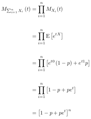
To identify the distribution of the sum of IID Bernoulli random variables, we can look at the moment generating function (MGF) and show that the sum of IID Bernoulli random variables and the Binomial random variable are the same:

The last line is a moment generating function for the Binomial random variable with mean np and variance np(1-p). Using this knowledge, we can then look at the probabilistic argument for consistency. Unfortunately, using the probabilistic statement directly is a challenge as we also need to understand the distribution of the absolute value of the estimator. That’s something I would never attempt for this problem. Instead, we rely on a well-known probabilistic relationship, called the Chebyshev Inequality.

Chebyshev Inequality

The Chebyshev Inequality is a relationship that bounds a probabilistic statement in a particular form:

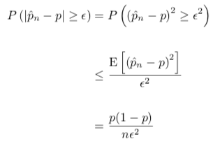
This is a particular form of the Markov Inequality, but allows us to identify convergence through the use of the variance associated with the underlying variable of interest. Therefore, writing the probabilistic argument for convergence, we see:

Applying the limit (increase in sample size), we see that the result goes to zero! Therefore, our estimator is indeed consistent!

Interpreting Consistency

Consistency is a limit-based argument. This means that it’s a theoretical value that will never be achieved in practice. To this end, we identify that our estimator indeed converges, and we are given some guidance as to how well it converges, thanks to the Chebyshev Inequality.

One way to interpret this relationship is that epsilon serves as a bound on the variance; and in turn, on the deviation of our analytic about the true underlying parameter of interest. We see this directly in the first line of the consistency proof for a coin flipping example. For argument’s sake, suppose the coin is fair; meaning the probability of obtaining a heads is one-half. Further suppose we are alright with obtaining variational error of one-percent. Then, the sample size required to ensure that we have these conditions met say 95% of the time is

which is 500.

This means we require 500 flips of the coin to ensure that our variance is within 1% at 95% probability. Taking this a step further, this translates to have 10% or more error on the estimator roughly 5% of the time… Yikes.

Let’s consider this from another context…

Three Point Shooting

We come back to our three point shooting argument before. Instead this time we look at it from the shooter’s perspective. The analytic question here is “How well does my player shoot from the perimeter?” If we see a player shoot 37% from beyond the arc, does that mean they are a 37% shooter?

Surprisingly, there has been little performed in this field. Darryl Blackport provided a quick treatise in reliability theory four years ago that involved the Kuder-Richardson 21 (KR-21) metric. For a while, a famous interview question from teams involved the dreaded “predict the three point percentage of every player in the league” which is, effectively an exercise in futility if you’re forced to get within 1 percentage point of truth. Over the previous few years, the rise of shot quality metrics have popped up to understand the quality of a shooter, which in turns leads to eFG+ calculations. However, this categorizes decision making first, and then relies on the same noisy statistic (field goal percentage from the perimeter) in measuring capability.

So let’s take a look at the KR-21 methodology.

Kuder-Richardson 21

The Kuder-Richardson 21 metric is a psychometric-based reliability measure to analyze the “quality” of a test given to students. The goal of the metric is to identify how consistent a test. The original application, from Kuder and Richardson’s 1937 paper, is to identify if two tests applied to the same student population are of equal difficulty. As such, the paper starts with a single test of many questions splits the test questions in half (at-random), treats them as two separate tests, and then computes the cross-correlation matrix of the test with n questions. The resulting cross-correlation score is called KR-1; the first equation of Kuder-Richardson.

The remainder of the paper introduces different scenarios and slowly develops a statistical framework for understanding the comparative quality of test questions. It is effectively a permutation test that ultimately results in an analysis of variance (ANOVA) by the time we reach KR-21.

The KR-21 equation is given by:

Here, sigma is the standard deviation of the test scores for each student and p is the proportion of students getting a single test item correct. Notice that the term np(1-p) is lingering in the equation. This is due to the fact that each question is been as a Bernoulli random variable and every test question is assumed to be of equal difficulty (and independent of all other test questions)!

Taking this a step further, since the Binomial distribution is now modeling test scores, we treat this as a basic regression problem and the resulting variance is a sum-of-squares for error while the sigma terms identify a total-sum-of-squares. Then we have:

which is indeed the ANOVA equivalent!

Application to Three Point Shooting “Ability”

Treating the KR-21 value as an ANOVA-like quantity, we effectively have an R-square calculation. Under R-square conventions, commonly the value of .7 is used as a “strong” value of correlation. Now to perform a KR-21 test, the challenge is to treat each player as a “student” who takes an “examination” of three point attempts. Ideally, we set the “number of questions” to be the number of three point attempts to be n. Then, for a collection of players who have taken n three point attempts, we compute the population variance of the players and the mean number of attempts across all players.

Starting at a small n, say 50, we collect all players across the league who have attempted 50 attempts and compute the KR-21 reliability number. If this number is too small (below 0.7), we simply increment n and repeat the study.

Unspoken Challenge: Are 3PM random?

One of the unspoken challenges with a reliability measure such as KR-21 is that we may obtain a negative reliability score. For example, let’s generate a sample of fifty shooters that each take 100 3PA’s. Suppose every 3PA is an IID Bernoulli random variable. Using rows as players and columns as 3PA, we obtain a chart that looks like this:

 

The green column is the number of made 3PA by that player. The yellow row is the number of 3PA made in that attempt number. By computing the SSE component from yellow, we obtain a value of 24.4976. By computing the SST component from green, we obtain a value of 17.6006. This leads to a KR-21 score of -0.3958.

Why did this happen? First of all, this is an okay result. A negative reliability score only indicates weak-to-no correlation between test items and users. Specifically, it doesn’t identify “equally difficult” problems; but rather yields “noisy” questions that are randomly solved. In the context of three point attempts, this would suggest all makes are completely random. Which, by definition of our exercise is exactly what had happened.

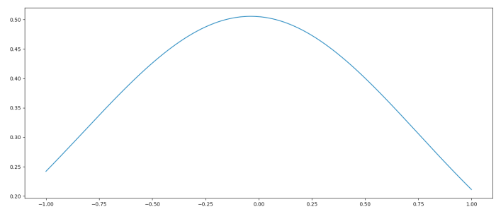
Now, if I change p=0.35, which was the league average for the 2018-19 NBA season, we see the exact same thing happen. This indicates that ordering every single player’s 3PA attempts matter significantly. In fact, we apply a MCMC simulation of KR-21 scores using the above set-up to identify the distribution of possible KR-21 scores:

What this exercise really tells us…

What this shows, for something along the lines of Blackport’s (and others in the Baseball community) analysis is that shooters continue shooting and others don’t. To be able to obtain a positive reliability score, shooters indeed have tendencies and they are picked up on within the KR-21 test. And once they are keyed in on, a value of n to nail down a high reliability number is approximately 750.

More importantly is that this shows that perimeter shooters scoring are not random events. Instead, they are indeed correlated scorers that have some frame of rhythm. If they do not, then a value of .7 reliability is never attainable except by random chance. Which, as you can see above, has exceptionally small probability.

Back to Consistency

So let’s go back to the Bernoulli coin flip problem. Instead of a coin, if we model a three point attempt as a Bernoulli process, we obtain the same probabilistic argument. Now suppose, using the worst case scenario of p=.05 (worst case means highest variance!), we note that 500 3PA attempts are required to nail down a 95% probabilistic true value with plus-or-minus 10% error. That’s incredulous.

If we impose a 1% error, we obtain instead require 50,000 attempts. Which is much less optimistic than the 750 attempts noted before.

No instead of the worst case scenario, we have the league-average of 35.5%, we (under the Bernoulli assumption) require 45,795 attempts to get within one percent error of truth at the 95% probabilistic level.

Leveraging the 750 number, we find that at league average levels, the actual margin of error associated with 750 attempts (bounded by probability) is really 1.8%. This is indeed a sweet-spot and reinforces the results obtained by Blackport from roughly five years ago. What this tells us is that there are indeed trends in shooting, but they are not strong as they are effectively within the variance of a Bernoulli process.

Now What…

To this point, we showed that three point percentages have weak trends, but can be modeled loosely as a Bernoulli random process. What this really tells us is that shooters attempt to optimize their perimeter scoring chances when they decide to shoot. This means attempts are not independent. Nor are they truly identically distributed. Furthermore, it’s difficult to obtain tight confidence regions on the true, underlying perimeter shooting percentage; which is why we see players fluctuate in rankings through the years.

To this end, there’s an underlying model for not only when shooters make attempts, but also for when they take attempts. At this point, developing a hierarchical model for the basic frequency-and-efficiency analysis. This way we can being to understand the player’s underlying decision making tendencies, in an effort to better understand their true underlying perimeter shooting capabilities.

In effect as Michael Scott once put it: “You miss 100% of the shots you don’t take. – Wayne Gretzky”

But as the moral of the story:  For every introduced analytic, there must be an adequate understanding of the variational properties related to the game. After all, the goal is to always get the signal above the noise.