Only a few days delayed due to an impromptu trip to Ottawa and a swing through Sacramento to catch the Kings upend the Minnesota Timberwolves 106-103 last night, my pre-season predictions are finally available for your viewing pleasure.

In this edition, we take a look at the rosters on opening day and compute their expected play per possession and simulate the entire season possession by possession. So in this edition, we return to form by building a model and describing the statistics used; and the present the results. So if you’re not into the math and statistics, jump below to RESULTS.

The Model: Building Weights for Player Performance

Now, with that out of the way, let’s take a look at our model. Given the 174,000-plus possessions last season we are able to break out each possession played by offense and defense with a rewards based system. Get an assist on offense? Get a point. Get a turnover on offense? Lose a point. If the player is on defense, they get the exact opposite score of the offense. In the end, each possession is measured by the number of positive plays minus the number of negative plays. So for instance, if there is a missed field goal, offensive rebound put-back dunk for two points, the scoring is as follows:

(-1 Missed FG) + (+1 Offensive Board) + (+1 Made FG) + (+2 Points Scored) = 3 Points

Now that every possession is scored, we have 10 players tagged to each possession; five with positive scores and five with negative scores. We also weight the interactions using three extra criteria: days since last game played, home/away location, and score differential compared to offense. These values are intended to identify impact between the players’ possessions and a basic environment of the game. We could add other factors such as amount of time played during game for each player and such; but we chose not to include more than 500 variables.

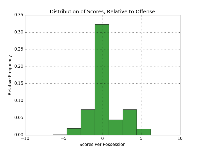
The distribution of scores is given by:

Applying a neural network, we obtain coefficients for every player with respect to the number of days between games, the point differential between two teams during the course of the game and the location of the game. These weights show how much contribution given to the game by that particular player. For the 2015-16 NBA season, the resulting top ten players are:

1. Klay Thompson – Golden State Warriors – 4.1273642
2. Paul George – Indiana Pacers – 3.973944
3. Chris Paul – Los Angeles Clippers – 3.422040
4. John Wall – Washington Wizards – 3.417769
5. LeBron James – Cleveland Cavaliers – 3.401085
6. Draymond Green – Golden State Warriors – 3.210094
7. DeAndre Jordan – Los Angeles Clippers – 3.199948
8. Kawhi Leonard – San Antonio Spurs – 3.184342
9. Stephen Curry – Golden State Warriors – 3.174495
10. Al Horford – Atlanta Hawks – 3.174366

We then take the opening day rosters and combine the scores of players from the previous years. Given the rosters as of the morning of Tuesday, October 25th, there were still 493 players on rosters. This amounted to approximately 16-17 players per team. Of the 493 players, 104 players listed had not logged a single possession the previous season. To account for these players, we use a random forest with previous statistics; college and abroad; to compare to other players within the league to approximate their contributing score.

The Simulation: Using the Model to Predict Player Performance

Now that we have a model, we can then simulate an entire season. Think of this like the NBA 2K simulation module; where players are given a particular attribute set and the game simulates statistics for each each based on the attributes. We do a similar thing by simulating every possession. To do this is relatively simple.

Consider we are simulating the Atlanta Hawks versus the Boston Celtics. The starting lineups would be the primary five players at each position; indicated by their position and weighting score. In this case, we would have:

Atlanta: Kent Bazemore, Dwight Howard, Kyle Korver, Paul Millsap, and Dennis Schroder

Boston: Avery Bradley, Jae Crowder, Al Horford, Amir Johnson, Isaiah Thomas

We take the players’ respective scores, their anticipated percentage of play (based on previous trends in seasons or random forest predictions),  and begin simulation using a coin flip to determine possession. Based on the contribution of the players, we have their relative statistics from the previous seasons and do the following:

Possession 1: (Boston Offense) Given the game is in Atlanta, both teams are on 1 day rest, and the score is 0-0; Atlanta’s five-player sum is 11.317843. Boston’s five-player sum is 12.189988. We form the ratio for each team to identify a positive or negative play. Boston has a 0.5188 chance of obtaining a positive play. We draw a random number and check if the number is below 0.5188. If yes, Boston has a positive interaction. In this case, we then break out the distribution of potential interactions that build a positive interaction based on the player set. In this simulation, Al Horford scores two points. Score: Boston 2, Atlanta 0; Rewards: Boston 3, Atlanta -3

Possession 2: (Atlanta Offense) Given the score is now 2-0 with anticipated 11:43 remaining in the first quarter; Atlanta’s five-player sum is 11.317854. Boston’s five-player sum is 12.188827. Same simulation process, we identify that Atlanta’s drawn a positive interaction. The break out based on the positive interactions is that Dennis Schroder missed a field goal attempt, Dwight Howard obtained the offensive rebound and scored two points. Score: Boston 2, Atlanta 2; Rewards: Boston 3, Atlanta 3.

Continuing in this process, the final score obtained is Boston 104, Atlanta 93. Stat leaders are Isaiah Thomas with 23 points and 7 assists along with Dwight Howard with 13 rebounds.

We merely continue this process for the remaining 1229 games.

Results: Predicted Records, Playoffs, MVP

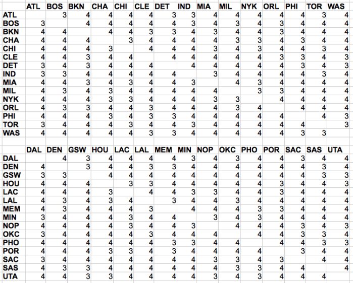
With the simulation process in hand, we first take a look at the schedule and identify that every team plays the opposite conference twice for a total of 30 games; their division 4 times for a total of 16 games; and the remainder of their conference a staggered 3-4 times. The distribution of games for every team (minus opposite conference) is given by

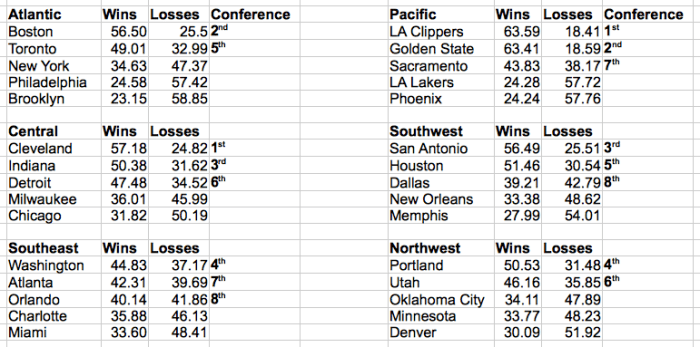
Using the season schedule, here are the predicted standings for the season:

This means the playoffs are given as follows:

1. EASTERN CONFERENCE
   1. Cleveland Cavaliers
   2. Boston Celtics
   3. Indiana Pacers
   4. Washington Wizards
   5. Toronto Raptors
   6. Detroit Pistons
   7. Atlanta Hawks
   8. Orlando Magic
2. WESTERN CONFERENCE
   1. Los Angeles Clippers
   2. Golden State Warriors
   3. San Antonio Spurs
   4. Portland Trailblazers
   5. Houston Rockets
   6. Utah Jazz
   7. Sacramento Kings
   8. Dallas Mavericks

The playoffs are predicted to be as follows:

• Eastern Conference First Round:
  • Cavaliers over Magic (4-0)
  • Celtics over Hawks (4-2)
  • Pistons over Pacers (4-3)
  • Raptors over Wizards (4-2)
• Western Conference First Round:
  • Clippers over Mavericks (4-1)
  • Warriors over Kings (4-1)
  • Spurs over Jazz (4-0)
  • Trailblazers over Rockets (4-2)
• Eastern Conference Second Round:
  • Cavaliers over Raptors (4-2)
  • Celtics over Pistons (4-1)
• Western Conference Second Round:
  • Clippers over Trailblazers (4-2)
  • Warriors over Spurs (4-2)
• Eastern Conference Finals:
  • Cavaliers over Celtics (4-2)
• Western Conference Finals: 
  • Warriors over Clippers (4-3)
• NBA Finals:
  • Cavaliers over Warriors (4-2)

The decision of who MVP would be would be a cross between statistics and the final standings of the team. Then a probability is given through a ranking algorithm that gives the following top five MVP candidates:

1. Chris Paul – Los Angeles Clippers 17.21%
2. LeBron James – Cleveland Cavaliers 16.37%
3. Isaiah Thomas – Boston Celtics 12.20%
4. Steph Curry – Golden State Warriors 9.99%
5. Russell Westbrook – Oklahoma City Thunder 5.31%

The remainder of the percentages are effectively spread across another 27 players (Kyle Korver has a 0.000001% by the way).

The Quality: How about last year?

We did this simulation last year. Here’s how we did.

• WESTERN CONFERENCE Predictions (Actual finish; Predicted Wins – Actual Wins)
  1. Golden State Warriors (1; 61-73 )
  2. Houston Rockets (8; 53-41)
  3. San Antonio Spurs (2; 52-67)
  4. Los Angeles Clippers (4; 51-53)
  5. Oklahoma City Thunder(3; 50-55)
  6. Memphis Grizzlies (7; 47-42)
  7. Dallas Mavericks (6; 42-42)
  8. New Orleans Pelicans (12; 41-30)
  9. Utah Jazz (9; 41-40)
  10. Phoenix (14; 39-23)
  11. Portland Trailblazers (5; 36-44)
  12. Sacramento Kings (10; 32-33)
  13. Denver Nuggets (11; 31-33)
  14. Los Angeles Lakers (15; 25-17)
  15. Minnesota Timberwolves (13; 21-29)

 

• EASTERN CONFERENCE Predictions (Actual Finish; Predicted Wins – Actual Wins)
  1. Cleveland Cavaliers (1; 53-57)
  2. Chicago Bulls (9; 51-42)
  3. Atlanta Hawks (4; 50-48)
  4. Washington Wizards (10; 49-41)
  5. Boston Celtics (5; 45-48)
  6. Milwaukee Bucks (12; 43-33)
  7. Toronto Raptors (2; 42-56)
  8. Indiana Pacers (7; 42-45)
  9. Orlando Magic (11; 40-35)
  10. Detroit Pistons (8; 38-44)
  11. Miami Heat (3; 38-48)
  12. Charlotte Hornets (6; 32-48)
  13. New York Knicks (13; 29-32)
  14. Brooklyn Nets (14; 29-21)
  15. Philadelphia 76ers (15; 25-10)

We see that some predictions were fairly off; but this is due to the model set-up. For starters, we cannot predict when Dwight Howard quits on a team like he did in Atlanta this past season. We also cannot predict when Marc Gasol will break his foot like he did in Memphis or Jabari Parker in Milwaukee. Nor tackle any other roster moves like trades or dumping of players like the Phoenix Suns, Philadelphia 76ers, and Milwaukee Bucks. Also, as a Markov Simulation, we tend to be conservative so that a 70 win season will rarely be predicted; and similarly a 15 loss season will rarely be predicted.

That said, the simulations managed to get 7 teams correct for making the playoffs in the Western Conference and 5 teams correct for making the playoffs in the Easter Conference. For predicting the number of wins; we had 14 teams within 1 standard deviation of prediction (5 games). Within 2 standard deviations, we had 23 teams correct. At three standard deviations, we predicted all teams correctly.

Of the 16 teams that got into the playoffs, the Eastern Conference Finals was predicted to be the Cavaliers over the Hawks 4-1; the Western Conference Finals was predicted to be the Warriors over the Spurs 4-3. The NBA Finals was predicted to be the Warriors over the Cavaliers in 4-3.

Warning, some theory here: The MVP selected for last year was most likely LeBron James. This did not happen either. This is due to the fact that probabilities have a large variance relative to their value. In response to my latest simulations for the world series (which on of the two teams in the series was predicted and the other team is the team that eliminated the predicted team) the most common response was “isn’t the variance suppose to be small?” Well let’s take a look…Suppose I have three options to win MVP. All have equal probability. Then each have a 1/3 chance. The error for each is just 1/3*2/3, which is 2/9. The ratio of the variance over the expected value is 2/3. Now if I have 20 options and a uniform distribution, then the mean is 1/20 and the variance is 1/20*19/20, which is 19/400. The ratio of the variance over the expected value is 19/20. Note that 19/20 is much larger than 2/3. This means that the maximum value, while has the highest probability, the options nearby are just as feasible to be selected; IE: 8% > 7% but 7% option can happen in a real-event one-time-only situation. 

So what do you think? Who’s the best teams in the league? Agree or disagree? What’s your model?