The terms offensive rating and defensive rating refers to the amount of points scored by a team and by the team’s opponents, respectively, over 100 possessions. The normalization to 100 possessions allows for the ability to compare teams as pace of games can skew points per game comparisons. Both ratings are still considered box score statistics as they rely purely on box score statistics. While the formula is simple, there is an estimation requirement as the number of possessions must be calculated from box score data.
With access to play-by-play data, we can focus on properly computing the number of possessions. For a refresher, feel free to review the definition of a possession and how they are grossly overestimated by NBA possession models. Since possessions are largely overestimated, the announced offensive and defensive ratings are lower than their true values, presenting bias in the presented results, and therefore making it undesirable to compare teams (or players if ratings are used at the player level) between years.
Once we correct for the actual number of possessions, we can then start looking at the nuances of offensive and defensive ratings. For instance, can a team lose a game despite having a higher offensive rating? The answer is yes. Similarly, if a team has a higher offensive rating than another team is the offense truly better? The answer is no. In this article, we walk through offensive and defensive rating, look at a distributional representation to show how we can compare teams, and present illustrations to actually compare teams. We will focus on play-by-play data spanning over the 2018 NBA season up through November 24th.
Case Study of Overestimation: Boston Celtics (17-3)
We select the Boston Celtics as our case study as they currently hold the “best defensive rating” of 96.8 according to NBA stats. The question is if they, in fact, really hold opponents to 96.8 points per 100 possessions. First, let’s apply NBA’s estimation process to each game and compare it to truth.

Game by game comparison of Estimated Possessions and Estimated Ratings to Actual Possessions and Actual Ratings.
Note that some games: New York Knicks, Golden State Warriors, and Miami Heat have more than five possessions of discrepancy between them. It is physically impossible to obtain this difference in possessions according to the definition of a possession from the NBA. While this is a problem with estimating possessions, the bigger problem is that most possessions are overestimated. In the possible forty possession counts, only one was underestimated: 93.88 possessions against 94 actual against the Knicks. All others? Consistently 4-6 possessions overestimated.

Plotting all the possessions from the 20 Celtics games, we can easily see the overestimation from the NBA possession model. This, in turn, translates into drastic differences between Offensive and Defensive Ratings between teams.

Comparison of Offensive Ratings (Blue) and Defensive Ratings (Red) using Estimated Possessions (Solid) and Actual Possessions (Dashed)
Comparing the distribution of Offensive Ratings and Defensive Ratings, we see that the overestimation in possessions dominoes into underestimating ratings. This is shown by the shifts to the right when comparing estimated ratings (solid lines) to the actual ratings (dashed lines).
What this really means is that the NBA reported 103.7 offensive rating and 96.8 defensive rating are actually 110.4 and 101.2, respectively.

As of this morning on the NBA Stats website. Note that the ORtg is 103.7 and DRtg is 96.8; which matches to the estimated model noted above with 103.74 and 96.79, respectively.
What this also means is that Boston Celtics opponents score more than one point per possession. In fact, Every NBA team gets more than one point per possession when we actually count possessions. Furthermore, the Celtics outscore opponents by 9.2 points per 100 possessions rather than 7.0 points per 100 possessions.
Now, if we use Offensive Rating and Defensive Rating to rate teams, what does this correction means for the rankings?
Ranking Teams Using Offensive and Defensive Ratings
Before we start correcting team rankings, we first take a look at the estimated rankings. As of this morning, NBA stats states that the rankings using offensive ratings are given by:

However, using actual possession counts, we find the list is somewhat out of order:
Thanks to an outrageously high scoring effort last night from the Golden State Warriors with a 143 – 94 win over the Chicago Bulls, the Warriors moved from second in the actual list to first in the actual list. In fact, the New York Knicks are not 10th in scoring per 100 possessions, as according to NBA stats, but rather they are 5th in the league.
Now, if we compared the Warriors and Rockets offense, based on Offensive Ratings alone, we would state that the Warriors are the better of the two teams. However, this required the Warriors to drop a large amount of points on one of the worst defensive teams in the league. If we removed the Bulls game, the Warriors would have an offensive rating of 116.84, which is less than the Houston Rockets’ 117.71.
What this suggests is that simply using ratings to rank teams is not robust. In fact, we obtain situations where teams have winning records such as the Minnesota Timberwolves (11-8) but get outscored by opponents 112.62 to 113.21. This particularly happens due to averages being non-robust estimators. For the Timberwolves, they have participated in large varying ratings (blow outs) games; for better and worse.
However, despite blow-outs messing up averages and the resulting ordering of teams, we also find that at the single game level, having a higher offensive rating than a defensive rating does not necessarily mean the offense wins the game.
We outscored the Opponent… And Lost
Of the first 276 games of the NBA season, there have been nine games where a team has a positive net rating but lost the game. It happened in both opening night games.
Cleveland 102, Boston 99
On opening night, the Cleveland Cavaliers obtained 98 offensive possessions to Boston’s 95 possessions. If both teams had exactly 100 points per 100 possessions, or one point per possession, then the final score should be 98-95, Cleveland. In order for Boston to catch Cleveland, they must score at least 3 extra points over their 95 possessions. Suggesting that they could score up to 100*(98 points /95 possessions) to get 103.16 points per 100 possessions and still lose.
Using this illustration, the Cavaliers finished with an offensive rating of 104.08. In order for the Celtics to even tie the game, they must have maintained an offensive rating of 107.37! Since the Celtics only managed 104.21 points per 100 possessions; they did not meet the requirement to win and lost despite scoring more per possession than their opponent.
Not an Epidemic to Any Team
While this happened to the Celtics, the Celtics have never been a participant in this situation ever since. In fact, over the nine games, this phenomenon has happened to 16 teams; only Cleveland and Minnesota being second offenders. Cleveland being the winner in both situations while Minnesota split the pair.
Here’s the a list of all the games that have been affected by the ORtg > DRtg but lost phenomenon:

Comparing Teams Using Their Distributions
Finally, we can start comparing teams based on their distributions of offensive and defensive ratings. To do this, we can assume something boldly naive and assume that ratings follow a Gaussian distribution. If we take a look at the density plots above; particularly the dashed lines, we find that defensive ratings for the Boston Celtics are effectively Gaussian, however offensive ratings are definitely not. This means, even if we extrapolate to the full league, we are giving up some information by assuming a Gaussian distribution. That said, using this as an illustration will help us for when we want to do this for real.
Bivariate Gaussian Distribution
Before we start comparing teams, let’s focus quickly on the Gaussian assumption. Here, offensive and defensive ratings are being viewed as a bivariate random variable. That is, there are two random variables for each team. While having a higher offensive rating than defensive rating does not necessarily mean a win, we can point to the low frequency of such a phenomenon happening and integrate the distribution below a “break even” line to estimate the likelihood of a team winning.
This means we must understand the distribution function for the bivariate Gaussian distribution; as this distribution is modeling our offensive and defensive ratings. The distribution function is given as

Let’s break this down quick. First, the values of x and y are offensive and defensive ratings, respectively. This means that mu_x and mu_y are the average offensive and defensive ratings, respectively. Similarly, sigma_x and sigma_y are the standard deviations of the offensive and defensive ratings, respectively.
Finally, the value rho illustrates the correlation between a team’s offensive and defensive rating. If this correlation is exactly 1, then for every point increase (or decrease) of a team’s offensive rating, their defensive rating moves exactly a point increase (or decrease) as well. Translating this to basketball speak, the more a team scores per possession, the more they give up (exactly) on defense per possession. We consider this the Enes Kanter effect.
However, if this correlation is -1, then for every point increase in offensive rating, the defensive rating decreases by a point. This indicates that the teams with negative correlation tend to be in blowout victories and defeats.
Illustratively, the bivariate Gaussian distribution reflects the Gaussian distributions on both the offensive and defensive ratings. Their intersection with yield ellipses, stretched by the standard deviations in ratings and rotated by the correlations between ratings.

Illustration of obtaining an elliptical contour for the bivariate Gaussian distribution from Gaussians placed on both the offensive and defensive ratings.
Therefore, we should be interested in standard ellipses such as the 95% confidence ellipse for each team.
Golden State Warriors: Maximum Differential
Applying this distributional assumption to the Golden State Warriors, we can plot the 95% contour for their ratings distribution. We can then compute the “break even” line calculate which percentage of the distribution is underneath the line.

Warriors are 14-5, two green dots are covering each other.
The Warriors green dots (wins) are all below the break-even line. However not all the red dots (losses) are above the line. In fact, the Houston Rockets game mentioned above is barely below the break-even line.
As we calculate the area underneath the break even line, the Golden State Warriors have 62.96% of their confidence region in the positive rating differential. Also note that the resulting ellipse is oblong. This is due to the offensive ratings having a higher standard deviation than the defensive ratings. This identifies that the Warriors tend to have much better shooting days than others; as evidenced by some games being below 100 points and some games being higher than 130 points.
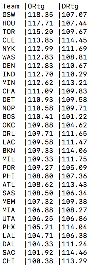
Comparison: Golden State vs. Houston
Now if we add the Houston Rockets to the mix, we can start comparing the two teams. By overlaying the two distributions, we gain insight into how the two teams operate over their first 18-19 games.
Don’t be fooled. Houston is red. However, overlaying with the Warriors, they look orange.
Here, we see that the Warriors distribution almost entire engulfs the Rockets’ distribution. What this indicates that the average offensive and defensive ratings are nearly equal, but the Rockets’ standard deviations are tighter. In fact, the Rockets have 64.24% of their distribution underneath the break even line, indicating that the Rockets are more capable of outscoring opponents over 100 possessions than the Golden State Warriors.
In fact, when matching these teams up, this would even indicate that the Rockets have a 51.37% chance of beating the Warriors, with an expected score of 118 – 116 over 100 possessions. Sounds a little familiar, doesn’t this?
Comparison: Golden State, Houston, and Boston
If we toss Boston into the mix, we find that all three teams are solidly below the break even line; as they are the three teams with the largest differentials.

We see that Boston is the tightest run ship of the bunch. Despite having the smaller ellipse, they have the highest below break even line probability with 68.55%. This indicates that the Celtics is indeed the top team when considering point differentials.
Summary Statistics for Every Team
Displaying every team’s pictures would be tedious at this point. Instead, we can display every team’s summary statistics: means, standard deviations, and correlation. This will give an insight into their elliptical distributions.
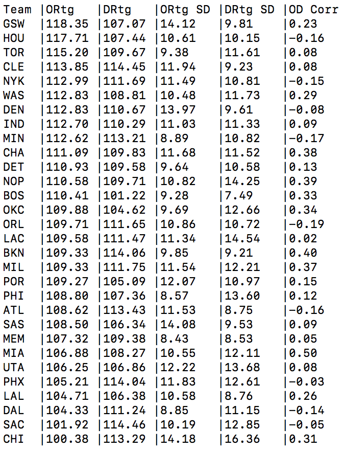
Sorted by average Offensive Rating.
Here, we see that every team is above 100 points per 100 possessions; thanks to corrected possession counts. We also see correlative phenomenons with teams such as the Warriors, Wizards, Hornets, Pelicans, Celtics, Thunder, Nets, Bucks, Heat, Lakers, and Bulls. These teams are in the camps of allowing more points as they score more points. To be clear, this does indicate that games are close, but rather that as a team scores more per 100 possessions, their opponent scores more per 100 possessions.
For example, the Warriors may typically outscore teams 118 to 107. If they score 125, their opponent may score around 114. Similarly, if they score 110, their opponent may score around 100.
That said, the Rockets, Knicks, Timberwolves, Magic, Hawks, and Mavericks all have negative correlations, indicating that they are typically blow-out teams; for better or worse. The Timberwolves, for instance, have endured at least four blow-out losses while handing out at least four blow-out wins. What this indicates is that these teams will either excell when building leads or implode when giving up points. These are the teams that tend to be volatile over the course of the season and are not likely to win an NBA championship, even if their record is relatively high.
Despite this, the season is early, and these numbers are close enough to zero that anything can change over the series of four games.
Comparing Teams Within Division: Atlantic Division
We leave off with a simple comparison of teams within a division. For this example, we complete the Boston Celtics thread and look at the Atlantic Division.

Color Scheme: Boston Celtics (green), Toronto Raptors (red), New York Knicks (orange), Brooklyn Nets (silver), and Philadelphia 76ers (salmon)
Here, we see that the Philadelphia 76ers (salmon) has a wildly large defensive variation. Due to this, the Sixers are a difficult team to rate above and below others. In fact, their below break even probability is 50.37%. This is a team that ratings wise should finish with 40-42 wins and may be on target for either 36 wins or 46 wins. All purely due to variability.
The Brooklyn Nets are also a curious case as they started out strong early in the season and their distribution has been slipping from below the break even line to above the break even line; as they are now being outscored by roughly 5 points per 100 possessions. Since the team is a fast-paced offense, looking at upwards to 100+ possessions, this does not bode well for the young team.
Given these distributions, we find that the Atlantic Division is one of the stronger divisions in the league when it comes to offensive and defensive ratings. In comparison, we can look at the Pacific Division and find that this is actually one of the weaker divisions in the league; thanks in part to the young teams of Los Angeles (Lakers), Sacramento, and Phoenix.

Color Scheme: Golden State Warriors (Gold), Phoenix Suns (Orange), Los Angeles Lakers (Purple), Sacramento (Violet), Los Angeles Clippers (Red)
In case you are unclear which ellipse is the Kings and which is the Lakers; the Sacramento Kings have the larger ellipse that points upward and rests almost entirely above the break even line. The Lakers are pointed to the right and is tightly compact near the break even line in the lower left of all the ellipses.
Comparing the two divisions, we see that while the Warriors are by and large the best team in the division (if not, arguably, the league), the rest of the division is not so hot. Every other team is below 50% when it comes to having a positive ratings differential.
What we are able to gain in insight here is how teams actually interact with their ratings and how we can actually use them to compare teams; as opposed to simply performing a sort. Furthermore, by correcting for possessions, we can actually start to compare teams from different seasons. While folks do this now with estimated ratings, those comparison must be taken with a grain of salt as possessions are grossly overestimated.
The question now is… how do we correct for season with no play-by-play data?


Pingback: Weekly Sports Analytics News Roundup - November 28th, 2017 - StatSheetStuffer
What libraries do you use to create these graphs?
LikeLike
These are MATLAB plots.
LikeLike