In 2002, Wes Colley (Princeton) developed a methodology that became a part of College Football BCS rankings lore: The Colley Method. In his original paper, Colley claims that his method is “bias free” for estimating the ranking of a team given a particular schedule. The resulting values for each team is identified as a ranking and therefore a realization from Laplace’s Rules of Succession. While basic statistics are misunderstood in the discussion yielded in Colley’s paper, two other problematic issues arise: there is an arbitrary weighting scheme and the resulting rankings, as governed by Laplace’s Rules of Succession, yield probabilities larger than one and less than zero. The latter portion is significant as it effectively states that teams can win more games than they participate in and win a negative amount of games, respectively.

In this article, we take a look at Colley’s methodology and attempt to understand the associated statistics with the procedure.

Consider One Team: Colley’s First Step

First, we start simple: let us only look at one team and their resulting wins and losses over the course of the season. Currently, the Atlanta Hawks have completed eight games into the season and have compiled a 1-7 record. The most basic model will consider each game as a random draw from a Bernoulli Distribution.

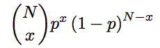
If you are unfamiliar, a Bernoulli distribution is a success/failure distribution for a given event. Here, an event for the Hawks is a game played. A win is considered a success, a loss is considered a failure. Then, we are interested in the probability of success, identified by the value p. The distribution for a Bernoulli random variable is given by:

The value, x, is merely and indicator of whether the Hawks won their game or lost their game. If we now consider every game as an independent Bernoulli trial, then we simply identify the number of wins as the sum of each x-value.

Now you may pause for a moment and ask, “doesn’t the probability of winning change from game to game?” While the answer to this is “YES!” we are interested in only the most basic model. We will expand on this in a bit.

Now, if we are to sum these 0 (loss) and 1 (win) events over N games, we obtain a Binomial distribution. A binomial distribution counts the number of successes (wins) over the course of N trials (games). There are a couple of key assumptions here:

1. Games have the same probability of success.
2. Each game is independent. Meaning back-to-backs don’t influence capability.

The distribution barely changes. In this case it becomes

 

In this case, we made a slight change. The value x is no longer 0 or 1; but rather is the number of wins in N games. For the Hawks, this would be a value between 0 and 8.

Estimating Success: Maximum Likelihood

A simple indicator of how well a team plays is to identify their probability of success. In reality, each team has their true value. In this set up, we don’t care about the opponents. Instead, we care only about the Hawks wins and losses. If we perform the maximum likelihood estimator for p, we are able to identify an estimated value of success for a team.

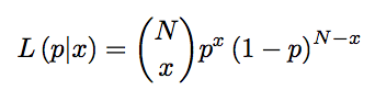
Maximum Likelihood is the process of taking observed data and computing the probabilistic model for the data evaluated at the observed data. This process is called building a likelihood function. We then maximize this function with respect to the parameter of interest. This will identify the highest probability of p from observing the data. In the general case, the likelihood function is the Binomial distribution. We then write the likelihood function as

 

One way to maximize this function is to take the derivative and set it equal to zero. We have to be careful and ensure that the second derivative is negative; or else we obtain a minimum… which is the lowest probability of p from observing the data. That would be bad. Here, we make a slight one-to-one transformation to make our life easier before we apply the differentiation. The resulting differentiation gives us

If we set this to zero and solve, we get

This is actually win percentage!!! This means that if we consider this ultra-simple set-up, the easiest way to compare teams is to look at a teams win’s percentage and call it a day. However, there are a lot of issues with this.

Filtering Success

One of the first issues we run into, particularly for small samples, is that the maximum likelihood operator has large variance and tends to be only a sample path of the actual state. This means the combination of both large variance and a single sample pass can give us wildly varying results in true probabilities of success. Instead, we might want to apply a filtering technique to control for spurious wins. To give example, during the Detroit Pistons versus Los Angeles Lakers game on October 31, 2017; with the Lakers handily ahead, the announcers made a comment that since the Detroit Pistons defeated the Golden State Warriors two days prior, that the Los Angeles Lakers are better than the Golden State Warriors. This flaw in transitive logic stems from the similar result above. If we isolate both games and apply straightforward win percentages, the Lakers are indeed better than the Warriors!

To remedy this, we apply a filtering technique. A common one is placement of a prior distribution on the parameter space. This is a Bayesian procedure that attempts to use prior information to control observed information, like we saw above. One of the requirements necessary for a prior is to have a domain identical to the domain of the parameter space. This means that if we put a prior on the probability of success, we obtain a value between zero and one.

The most common technique for the Binomial distribution is to place a Beta distribution prior on p. The formulation for a resulting posterior distribution is given as (Likelihood x Prior) / marginal. The marginal distribution is the normalizing constant of the posterior distribution. In this case, we have the posterior distribution to be:

Let’s break down this quantity and show that it’s not as scary. First, let’s factor out the terms that have nothing to do with the probability of success. These terms all cancel out! Next, let’s combine like terms. This leaves us with

 

You may recognize this. This is a Beta distribution but with the parameters updated by the observed data! The values of alpha and beta are used to filter the probability of success. The more important thing here is that if we compute the expected value, or posterior mean, we obtain an estimator for p given the data. In this case, the expected value is

This means the win percentage is stretched to a competing value by these parameters of alpha and beta. If we set alpha = beta = 1, we get the Uniform distribution! This means that every team is equal before the season begins, and as games are played, their resulting probability of winning changes from uniform. Let’s plus in one for both alpha and beta:

If you made it this far, congratulations! This is the starting point for Colley’s Method. Colley’s Method is the process of assuming that every team follows a game independent, unrelated to other teams, unaffected by schedule, with uniform prior building to estimated the probability of success for a team.

What does this mean for the Atlanta Hawks? Well, while their 1-7 record would give them a 0.125 win percentage, their filtered win percentage is 0.222. Meaning that they are simply on a sample path slightly worse than their actual probability of success.

From this point, Colley makes some subtle changes in attempts to incorporate scheduling and team-versus-team interactions. Let’s dive in finally!

Rewriting Number of Wins

One of the first steps that Colley performs of this posterior mean is to rewrite the number of wins for a team. This is a straightforward, but misleading, process! Instead of following Colley’s footsteps, let’s apply Colley’s ideas in the general sense.

First, we take the number of wins and write them as a weighted sum of wins, losses, and games played. This is given by

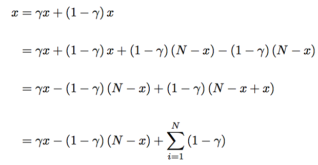
Let’s break this down. First, we split the number of wins into a gamma percentage of wins plus a 1-gamma percentage of wins. We then add and subtract in a 1-gamma percentage of losses. This is effectively adding zero and not changing the equation.

The third step collects like terms. The final term is 1-gamma times the number of games played! Since the number of games played is constant, multiplied to a constant 1-gamma, we can rewrite this as a sum. This means each game played by that team is identified by 1-gamma.

This means the final term is merely the weighted number of wins. The weighted number of losses. and the weighted strength of schedule. If we now return to Colley’s footsteps, Colley applies gamma = 0.5. In this case we obtain

This is effectively the win percentage given half weight and the strength of schedule being uniform across all teams, given half weight.

Different Weightings: Where Colley is Misleading

We can apply a different weighting scheme. Suppose I want to give only ten percent to strength of schedule. Then, all we need to do is set gamma = 0.9. This would give us

Ignoring Past Assumptions to Incorporate Strength of Teams

The next step in Colley’s Method is to change the underlying assumptions of uniformity. Ignoring the requirement, Colley replaces the 1/2 term in the strength of schedule to be r_i, or the ranking of team i. This leads to the equation for a win to be

This is now a single equation with q unknowns. Here q denotes the the number of unique teams played against by the, in this case, Atlanta Hawks. In an effort to build a linear system of equations, allowing us to solve for these unknown ratings, we now consider this equation for all teams.

Multiple Teams

To understand how all teams work, let’s index every team by index j. This means j=0 is the Atlanta Hawks, j=1 is the Boston Celtics, and so on. Then we obtain the system of equations identified as

There are a total of 30 of these equations, with 30 unknowns of r_i^j. The value, r_i^j just means the rating for game i opponent of team j. If we rewrite this in terms of a set of linear equations, we obtain the following:

 

 

Let’s walk through this. Line one is the original definition from the Beta-Binomial posterior distribution. Colley states that the posterior mean (probability of success) is indeed the team ranking score.

The second line substitutes in the rewritten line for wins; using the ignoring of the uniform assumption.

The third line rearranges the terms such that all the team rankings are on the left hand side, while the terms that do not contain the team rankings (constants) are on the right hand side.

Finally, the fourth line rearranges the sum to identify the number of times team j has played team i. Therefore we can walk the sum over all teams as opposed to all games!

What this now gives us in the following: For team j, we associate to them N+2 games. This is the filtered number of games from the Beta-Binomial distribution. For opponent i of team j, we associated -n_ij games. This is the number of games played between team i and team j. For team j, we associate the response to be 1 + (number of wins – number of losses)/2. Think of this as reflection of the win-loss ratio for the team.

Putting this all together we can obtain a matrix representation of this system of linear equations.

Matrix Representation

The matrix representation is given by

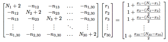
This is written in short form as Cr = b. Here, C is the schedule matrix. This portion identifies the strength of schedule for a given team. Each row is a team’s schedule with the diagonal being the number of games played (plus two with the Beta filtering), and the off-diagonal begin the number of games played against the opponent that the column represents.

The matrix (vector), b, is the number wins minus the number of losses (win differential) divided by 2. We add on the value of one from the Beta filtering. We think of each entry as effective win percentage for each team. To be clear, a .500 team results in 1 + 0/2 = 1, as the wins and losses cancel each other out.

Therefore the solution of rankings, r, is just the inverse of C times b. This is merely strength of schedule adjustment on the win-percentage. There is no closed form solution for the generalized matrix, C, and closed form solutions for the NBA is excessively messy. Due to this, we cannot identify explicit bounds on the rankings.

Instead, let’s look at a couple simple examples. This will help show some issues with the Colley rankings system.

Example 1: Four Teams, Two Conferences, No Out-of-Conference Games

Let’s start simple where we have four teams split evenly into two team conferences. For the league, a total of four games are played. Therefore each team plays their same opponent all four times. The resulting Colley matrix system is given by

Possible Finishes

There are a total of 25 possible outcomes for the season. Since the season is completely partitioned, we can focus on one conference. In this case, we identify the five following scenarios:

• Team A wins all four games: b_1 = 3, b_2 = -1
• Team A wins three games:  b_1 = 2, b_2 = 0
• Team A wins two games: b_1 = 1, b_2 = 1
• Team A wins one game:  b_1 = 0, b_2 = 2
• Team A wins zero games: b_1 =  -1, b_2 = 3

The other conference has the same breakdown.

Results

Now, if we invert the schedule matrix, we see how much weight the schedule places on the win-loss records for each team. Here, the inverse of the schedule matrix is given by

What this shows is that there is a clear conference bias as only in-conference games are weighted. We interpret that the schedule places sixty percent weight on the team’s win-loss record, while placing forty percent weight on the team’s lone opponent’s win-loss record. Therefore, if the two best teams are in the same conference, we could very well see them split games and finish 2-2. While in the other conference, one team is a complete cupcake, resulting in a 4-0 versus 0-4 record. Let’s mark these teams as A, B, C, and D, respectively.

This results in a b vector of [1, 1, 3, -1]. Multiplying by the inverse of the schedule matrix we obtain the rankings vector, r, as [0.5, 0.5, 0.7, 0.3]. A good sign is that we obtain all rankings between zero and one. This is not always the case in the general situation.

In this case, we find that Team C is ranked first despite never playing a difficult opponent. This is due to conference biasing through the scheduling (sampling frame). Therefore, let’s mix things up.

Example 2: Four Teams, Two Conferences, Half Out-of-Conference Games

If we change the schedule slightly and have two games in conference and two games out of conference, we obtain the following scheduling matrix:

In this case, it is impossible to obtain two undefeated teams. Instead we obtain more than 25 possible outcomes. While we still have less than 64 possible outcomes, there are 60 in total, we will not state all the use cases. Instead, we focus on the strength of schedule impact.

Inverting the schedule matrix, we obtain

Scenario 1: Best Teams in Same Conference

If we consider the old problem of the two best teams in the same conference and they split their two games, but win out of conference we obtain the following b vector: [1, -1, 2, 2]. This corresponds to a respective record set of: 2-2, 0-4, 3-1, 3-1. In this case, the rankings, r, are given by [0.46, 0.21, 0.67, 0.67].

This is the best scenario possible as we have a complete sampling frame of the entire league. We may have issues with ranking as Team A will be down weighted by Team B merely due to scheduling; however this is remedied by playing both Team C and Team D.

Example 3: One Out-of-Conference Game

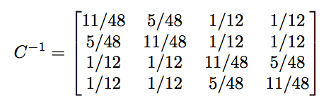
Finally, let’s look at another out of conference situation. In this case, we have three games in conference and one game out of conference. In this case, we can set the schedule matrix as

In this case, the inverse is given by

We see that there is now rating introduced to teams from teams they have never played. For instance, Team A obtains 11.25% of their ranking from a team they never played. If this team is poor, then Team A is penalized every time that team plays.

Scenario One: Team A is amazing

In this scenario, assume Team A is the best team in the league and every other team is mediocre. Then suppose we obtain a b vector of [3, 0, 0, 1]. This results in a record set of 4-0, 1-3, 1-3, 2-2. This results in a 128/160 = 0.8. The overall rankings are [0.80, 0.45, 0.30, 0.45].

Assumed Theory Violated!

What’s interesting here is that this is the first instance that the average of all rankings is not 1/2. This violates the expected requirement and is a result of the fractional sampling frame of the schedule.

Let’s verify this: Team A plays Team B three times. In the end, Team A is 3-0, Team B is 0-3. Team A play Team D while Team B plays Team C. This results in Team A 4-0, Team B 1-3, Team C 0-1, Team D 0-1. Team C plays Team D three times and this results in Team C 1-3 as Team D goes 2-2. This results in the b vector of [3, 0, 0, 1].

This shows that despite the assumed proof finding an average ranking of 1/2 in Colley’s paper, here is a counter-example that proves otherwise true.

Continuing Along These Lines: Probabilities Are No Longer Probabilities

If we have a larger schedule and large population of teams, we run into other major issues. For instance, let’s consider Week 14 of the 2011 NCAA Football schedule. In this case, the 2012 sampling frame (schedule matrix) yielded such a weighting that we obtained probabilities larger than one!

Note: Ranking is determined to be the probability of success as defined in equation 1 in Colley’s paper. Therefore it must be between 0 and 1.

This happens due to the fact the uniform distribution is used as the filter and later, the mean of the filter is thrown away in favor of a general mean. Since this general mean does not match the filtering distribution used, any scheduling bias will pull this filtered probability outside of possible ranges.

Conclusions

What this indicates is that Colley’s Method is schedule/conference biased as witnessed by penalizing a second best team due to scheduling (Examples 1 and 2), that the assumed weighting will result in a global mean of 0.5 is also false (Example 3), and that the ignored assumptions violate the definition of probability of success (Thanks LSU…).

The reason this all occurs is due to the fact that the original assumption is that every team’s sample path of games is independent of every other team! This was the very start of this article. Recall we focused on one team. This assumption is purely false and the correction should focus more on a graph-based/network approach.

With the weighted win-loss versus strength of schedule partition of wins, we obtain 30 independent equations. To impose the correlation between the teams played, the general values of r are injected without any pure rationale other than “it makes sense.” We have viewed above, despite conference biasing (which is an experimental design issue, not a Colley issue), we still require a carefully thought out sampling frame. In NCAA college football, this is not the case. For the NBA, we are fine as teams play everyone in their conference 3-4 times, everyone in their division 4 times, and everyone outside of their conference twice. Despite the distributional assumptions being incorrect, we still obtain an interpretation ranking.

Finally, Some Code

If you’d like to play around with your own Colley Matrix, here’s the associated Python code:

Through November 3rd, 2017

For the NBA, considering games through November 3rd, we have witnessed 130 total games played. The current records are given by:

The resulting Colley Rankings are given by

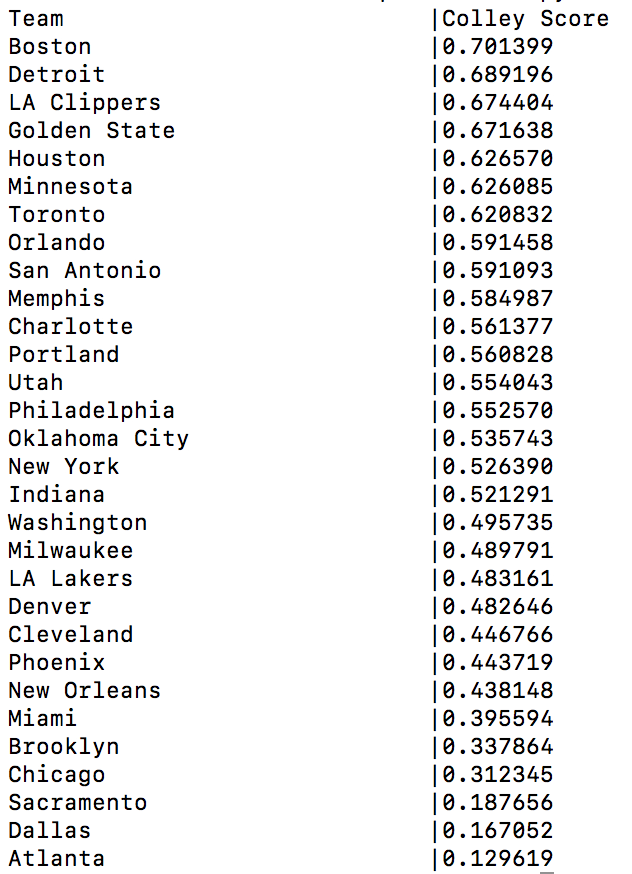
And Atlanta has since lost an 8th game since starting this article, falling to 1-8 and the bottom of the Colley Rankings.