The calculation for Offensive Rating, another fruitful Dean Oliver metric, is simple: compute the number of points produced when a player is in the game per 100 possessions that the player is in the game. The computation is performed at a “per possession” rate and scaled out to 100.

The challenge lies at being restricted to using only box-score statistics to compute these values. This has been a major challenge since we cannot simply count the number of possessions in a game using play-by-play data. Instead, a model must be devised to identify the number of possessions played. And even those models are consistently biased.In this article, we take a deep dive into Offensive Rating and attempt to understand the mechanics and statistical properties of the advanced metric.

Along the way, we will present simple Python code to compute Offensive Rating; which in turn will help you have existing code to make change to test out ideas in adjusting Offensive Rating.

Possessions Played

Total Possessions, as defined in Oliver’s “Basketball on Paper,” is an estimated quantity that identify when a team ends their possession. Possessions end when a field goal is converted, a final free throw is converted, a defensive rebound is secured, or a turnover has been committed. In these situations, end of possessions are ignored; which are usually heaves or other non-traditional or unplanned/desperate, basketball movements.

Possessions are then deconstructed into four primary components: scoring possessions, missed field goals that terminate possessions, missed free throws that terminate possessions, and turnovers. In this case, we should see exactly a four part representation of total possessions.

Before we dive into each of the four areas, let’s take a not as to what each component means. This is by far going to to turn complex very quickly. The goal in determining the number of possessions is to identify the possessions that a player in question is able to make an impact. To do this, we take the distribution of the team and identify how the distribution changes with respect to the player in question. Since we are limited to box-score statistics only, this becomes an exercise in aggregated sampling and borrowing strength statistical representations. In this vein, scoring possessions in particular, will have a complex interaction of various statistics. In fact, here’s the complicated flow chart of how Total Possessions is computed.

Scoring Possessions

The difficult part of this computation belongs to scoring possessions. These are possessions for which scoring a point terminates the possession. Note that this is not all terminating scoring possessions as teams can score points and finish with a missed field goal or missed free throw.

Scoring possessions are broken down into a series of four parts as well: Field Goals, Assists, Free Throws, and Offensive Rebounds. Each of these parts contribute to either directly scoring, or keeping the ball alive to continue chances of scoring. However, it’s not as simple as just adding these values; as they do not insinuate terminating possessions directly. For instance, made field goals can either lead to a terminated possession or a continuation foul. The continuation extends the possession, which either leads to a free throw terminating the possession; or in light if an offensive rebound, an extended possession.

 

Here, the only box score statistic introduced is Team Offensive Rebounds. In order to understand this quantity, we must work backwards up the flow chart in efforts to piecemeal the Scoring Possession quantity.

Team Scoring Possessions: TeamSCPoss

Team Scoring Possessions are situations where possessions end due to field goals. The quantity is defined by

This is relatively easy to break down. TeamFGM are the number of made field goals made by the team, regardless of two or three point attempts. Taking a look at the square term, we actually have percentage of missed free throws. Now if we square this term, we get an interesting breakdown:

The first term is merely the percentage of free throws that are made. The second term is the variance of a Bernoulli trial for team free throws! When multiplied by TeamFTA, we have ourselves the observed number of free throws made plus the variance of a Binomial distribution on Team Free throws made.

 

Let’s be careful here as the intent of this value is not what we described. The intent is that this is also the two-free-throw Binomial probability of making at least one free throw. As it is a probabilistic statement using its maximum likelihood estimator, we obtain this variance representation. This allows us to directly calculate expected values:

The multiplier of 0.4? This is a value determined roughly a decade ago to identify the percentage of free throws that terminate a possession. This multiplier is well-outdated as it has been updated to 0.44 by the NBA; and even then, is a free-flowing statistic that changes often (approximately 0.42 plus-minus 0.02) every year.

In the end, team scoring possessions are determined as possessions terminated by scoring: made field goals and expected number of possessions where free throws were made on possession ending free throw situations.

Team Played Offensive Rebound Adjustment in Scoring Possessions

Once Team Scoring possessions are counted, we must calculate the quantity (1 – TeamOREB / Team SCPoss). Once we realized that Team Scoring Possessions are looking for possessions that ended with points, this quantity comes into focus. This quantity attempts to measure the percentage of Team Scoring Possessions with offensive rebounds removed. This is an attempt at partitioning offensive rebound contributions at a later time. The issue here is that we can get negative contributions:

In order to see this, we identify that there merely needs to be more offensive rebounds than scoring possessions. As offensive rebounds cannot be gathered on made field goals, these are possession situations where offensive rebounds come on missed final free throws. For instance suppose there is a possession where two offensive rebounds are made and only one of four free throws are converted. Then the associated scoring possession is listed as 0 + 0.4*(1 – (1 – 1/4)^2)*4 = 7/10 = 0.70. With two offensive rebounds, we have a percentage of scoring possessions without an offensive rebound being 1 – 2/.7 = -1.3/.7, which is approximately a negative 200 percent.

Fortunately, games are not played at a fourth grade recreation rate and this probability indeed settles within (0,1). However, its statistical distribution does not.

Team Play Percentage

This quantity is simply the number of scoring possessions divided by the number of possessions played. In this case, the crude FGA + 0.4*FTA + TOV calculation is applied. While it has been seen that this formula is upwards of hundreds of possessions off, this is the possession model used. In this case we obtain percentage of possessions that result in points scored.

Team Offensive Rebound Weight

The team offensive rebound rate requires the Team Offensive Rebound Percentage and the Team Play Percentage. In this case, the team offensive rebound percentage is merely the percentage of offensive rebounds obtained from the total number of possible rebounds on an offensive possession: OREB / (OREB + Opponent DREB).

In this case, team offensive rebound weight is given by

Breaking this down, the numerator is immediately seen as the percentage of scoring possessions that resulted in a defensive rebound for an opponent. This is identified as 1 – TeamOREB% is merely opponent defensive rebound percentage. Multiply this by the percentage of possessions being scoring possessions and we have the probability that a possession ends with points scored and a defensive rebound for an opponent.

For the denominator, we have the numerator, but also situations where the team obtains an offensive rebound when possessions are not scored on. What the denominator attempts to capture are situations where points are scored but the defense rebounds the ball and situations where no points are scored on the possession but offensive rebounds are obtained.

Constructing this fraction helps us identify a weighting scheme that will help partition offensive rebounds into scoring and non-scoring opportunities. Similarly, this attempts to partition defensive rebound situations where points are still scored, as opposed to points not scored.

Now that we have the multiplier in hand, we can attempt to better understand its purpose in light of scoring situations.

Field Goal Part of Scoring Possessions

The field goal part of scoring possession is an attempt to identify the points produced by a player with respect to field goals made. This value is given by

The quantity qAST is the challenging part. First off, we identify the number of field goals made by the player of interest. The quantity PTS – FTM is merely counting the number of points scored on field goal attempts. Dividing by FGA and multiplying by 0.5 yields Effective Field Goal Percentage. This is seen as PTS = 2*FGM + 3PM leads to 0.5*PTS = FGM + 0.5*3PM, with eFG% = (FGM + 0.5*3PM)/FGA. This means we can rewrite the Field Goal Part as

Now, we need to understand this qAST term.

Assist Adjustment Factor

The assist adjustment factor is a correction factor that attempts to identify the biases between a player and their respective team. It is given by the formula

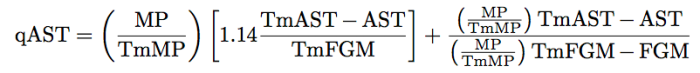
There are three terms to break down here. First, let’s look at the numerator on the second additive term. The fraction MP / Team MP is merely the percentage of minutes played by a player of interest. When we multiply this against the number of assists by the team, we obtain the expected number of assists for that player. For instance if a team obtains 2000 assists over the course of the season and a player obtains 10% of the season; that player should be expected to obtain 200 of the team’s assists. By subtracting, we obtain the bias in assists between the player and their team.

In the second term of interest, the denominator of the second additive term, we obtain a similar construction as the numerator. In this case we obtain the bias in field goals made between a player and their team. In this case, if a player does not get many assists, this quantity will balloon if they do not score many points either. However, if the player is a scorer, they negate not being an assist-type player as they are the ones scoring.

The first term looks at the percentage of field goals made that were the result of an assist not by the given player. An extra 1.14 multiplier is hard-coded in; without an understandable interpretation. As 0.4 was the rough estimate of percentage free throws that terminate a possession; the 1.14 here would indicate that fourteen percent of field goals made could not be obtained via an assist. Therefore the rate of assists to field goals is expanded to 114%.

Therefore we can identify this quantity as percentage of field goals assisted by teammates while the player of interest is in the game plus the expected rate of assists per field goals made for the player of interest. Here, we have partitioned assists into teammates and the the player themselves. This value can be rather large for a player who rarely scores and can be negative for players who rarely get assists.

However, placed back into the Field Goal Part, this becomes a multiplier on the effective field goal percentage. This in part attempts to partition field goals into field goals obtained through assists and fields that are just made. The idea here is to included assists through the assist part of the scoring possession.

Assist Part of Scoring Possession

The assist part of Scoring Possession is given by

Here, the numerator is merely the points scored by the rest of the team on field goals. The denominator is two times the number of field goals attempted by the team. With a little algebra, we see that this is merely the effective field goal percentage of the rest of the team.

This amounts to the weighted amount of assists with respect to effective field goal percentage. The one-half value is use to offset the one-half value in the Field Goal Part.

Therefore the FIELD GOAL part and the ASSIST part of the SCORING POSSESSION is merely the number of field goals made by the player PLUS the point contribution of the player through assists to the rest of his team MINUS the points contribution of the player coming from his teammates MINUS the rate of assists that the player should have made compared to the rest of his team.

Note that this is not counting the number of points produced, but rather the roughly number of field goals converted; as we are interested in possession counts where scoring occurs.

Free Throw Part of Scoring Possessions

The Free Throw portion of Scoring Possessions is the simplest, yet most egregious of the bunch. Here, we have once again a Binomial distribution of two free throws as we count the expected number of possessions where free throws are scored. This assumes that there are always two free throws and that 40% of free throws terminate possessions. (For the 2017 NBA season the maximum likelihood estimate was 0.434).

Offensive Rebound Part of Scoring Possessions

The offensive rebounding part of Scoring Possessions is simply the number of team rebounds multiplied by the Team Offensive Rebound Weight and the Team Played Percentage. Here, offensive rebounds continue a possession. Multiplying by the Team Play Percent gives situations where points are scored with offensive rebounds occurring. Multiplying by the Team Offensive Rebound Weight, we obtain the percentage of possessions where points are scored with offensive rebounds and defensive rebounds terminating the possession. These are typically situations where offensive rebounds lead to shooting fouls that have a missed last free throw rebounded by the other team. This actually happens more often than one would think in the league.

In this case, this quantity captures these instances and counts them towards scoring possessions. This quantity also makes up for the Field Goal Part, Assist Part, and Free Throw Parts having scoring possessions with offensive rebounds discounted.

Putting these terms together help yield the number of possessions where at least a single point has occurred.

 

Field Goals Missed Per Possession

The second component in determining the total number of possessions is the field goal per possession quantity. This value is simply calculated as (FGA – FGM)*(1 – 1.07TeamOREB%).

These are situations where a missed field goal results in an end of possession. As the previous (and painfully long) calculation of scoring possessions occur, here we must assume that no points were scored in this possession. Therefore we first identify the number of missed field goal attempts by the player. This is FGA – FGM. We then take all misses and multiply this by the percentage of missed field goals that are defensively rebounded. In this case, there is a multiplier of 1.07 used. This multiplier assumes that 7% of rebounds that return of the offense are not offensive rebounds. These are typically team rebounds that go off the hands of defenders after a missed shot attempt. The rate seems particularly high, however there are always rebounds up for grabs after blocks; particularly blocks out of bounds.

Multiplying these two quantities together yield possessions where a player has missed a field goal and the opponent ends up with the basketball.

Free Throws Missed Per Possessions

Similar to field goals missed per possession, free throws per possession again assumes a Binomial distribution with two free throw attempts. In this case, we are interested in no points being scored. This means our quantity is now 0.4*FTA*(1 – FTM / FTA)^2. The squared term is the probability of missing both free throws. Multiplying by the number of free throws attempted gives the expected value of missing both free throws, or number of pairs of free throws that result in an 0-for-2 situation. Multiplying this by 0.4 gives the expected number of final free throws being missed, when no points are scored.

Turnovers

The final value of Scoring Possessions are situations that end in turnovers. In this case, we have a curious situation as a turnover can occur after a field goal attempt in a possession. However, they are not accounted for in correcting scoring possessions. One question may be to ask is: “How many situations has a team turned the ball over on a possession after scoring and obtaining an offensive rebound?” If this answer is zero, we have ourselves a non-starter of a question.

Points Produced

Now that we have walked through Oliver’s methodology for partitioning the number of possessions a player has played in, we then turn our focus to how many points are produced by the player of interest. This quantity attempts to actually count the points, whereas above we were interested into only identifying possessions played.

Similar to Scoring Possessions, Points Produced has four parts to it: Points Produced off Field Goals, Points Produced off Assists, Points Produced off Free Throws, and Points Produced off Offensive Rebounds.

Points Produced off Field Goals

For field goals, we have the formula

The first term multiplied by 2 is actually Points Scored. Through the second term, we subtract the effective field goal percentage scaled by the assist adjustment from above. This is to capture points scored by the player, but were generated by teammates. This allows us to incorporate points generated through assists, but still have meaning when scaled to 100 possessions. Without the assist adjustment, we will see Offensive Ratings upwards of 150 points per 100 possessions; which is unreasonable.

Points Produced off Assists

Points produced off assists attempts to capture the point production from players who pass to score. While they are not the primary scorers, these players are typically the players who identify open passing lanes, or find ways to get a scorer open for a look. Here, the formula is given as

There are two primary terms of interest here. The first term identifies the looks at the field goal distribution of made field goals of the rest of the team, or with the player of interest removed. Applying a little algebra, we see that this is

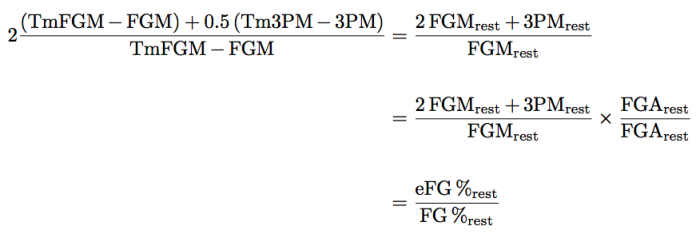
which is merely the difference in effective field goal percentage to field goal percentage for the rest of the team. If this player is a solid three point shooter, expect this to be small. If the shooter is not a three point aficionado, expect this to be large.

The second term we have seen before. This is effective field goal percentage as well. Combining these two terms, we obtain

This is the contribution of points scored off an assists. The scaling of eFG% / FG%
just attempts to obtain a relative point offset for the assist. The one-half is the half contribution (scorer and assist man) to the points being scored.

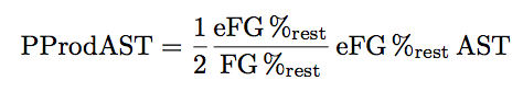
Points Produced off Offensive Rebounds

The final part of the Points Produced calculation is to look at the impact of offensive rebounding on scoring. The formula looks a little complex, but it is manageable:

Let’s start with the ugly fraction first. The denominator is the computation of “possessions” of points scored. The (1 – (1 -p)^2) term we have seen before. This is that same old Binomial distribution term with two free throw attempts running around. This term is simply calculating the probability that at least one free throw is made. Multiplying by FTA gives the expected number of free throws made; and the 0.4 construct is that same hard-coded value that suggests 40% of free throws terminate a possession. Therefore this ugly fraction calculates the points per possession when a point is scored. Multiplying this by TeamPlayPercentage yields the percentage of plays that result in points scored. Therefore we have a rough estimate of the number of points scored per possession. The Team Offensive Rebound Weight identifies possessions that should be rebounded by the defense. This results in points per possession that the defense should have rebounded. In this case, we multiply the number of offensive rebounds to identify the number of points scored per possession when an offensive rebound occurs and it should have been rebounded by an opponent.

 

And…. Offensive Rating

Once we obtain these parts, we finally obtain

Using the flow chart and understanding how this quantity is calculated, we realize that there was a lot of effort placed into solving a constrained optimization problem here. The constraints were the coarse box-score values of a player. And an iterative process, such as partitioning possible outcomes were used to hopefully estimate varying scenarios.

For instance, if a player had three offensive rebounds how do we know if they all came on the same possession? We don’t with box score data. With the release of play-by-play data, much of these parts can be simply counted. For instance, the number of possessions.

That said, this calculation allows us to compare players from the era before play-by-play data and gives insight on how to attempt estimation of fine-tuned parameters when only coarse data exists.

And Now for a Bit of Python

If you have made it this far, congrats! I’ll unleash the Python code. If you skipped right here; buyer beware! Using code without understanding its properties can be perilous. I encourage you to go back and attempt to understand the rationale on why the things performed in Offensive Rating is performed. This will hopefully shed insight on how to improve Offensive Rating; or better yet, identify how you would go about constructing a similar metric.

Data, data, data

Box score data is the simplest to obtain. Basketball Reference is a great place to get summary statistics. So is NBA Stats. Just be sure to follow their terms of usage. For instance, don’t download their data and attempt to profit off it it without their consent!

Once you have such data, you can store them as comma separated value files and proceed accordingly.

Let’s start by import pandas as pd and then bring in the files. Note, I left my directory hidden. Just point to your own directory where the files are stored.

Creating Output

Notice that I built a template. That merely helps me output data. If you recently have seen my Titter feed @squared2020, you would have seen such output already. Similarly, I keep two arrays open to look at plots later; these arrays are ORatings and usages.

Iterate through Rows and Compute the Formulae Above!

Now we walk through that flow chart above and make sure to compute the quantities in the correct order.

Note that grabbing a single value for a player is simply calling their statistical category. Each row is a player. To identify the team played, we call a secondary key of teams.Name, where teams is the team summary stats file. Continuing on within the same for loop:

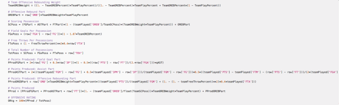
Unfortunately, we omitted the tail of the PProdASTPart line due to screen capturing capability. This part is just long from all the category calls. However, you should be fine in finishing the line of code (two terms are missing) .

The final line is simply the Offensive Rating.

Results

If I include a single check at each player row of data, I can output certain players. For instance, I can look at all players who played in more than seventy percent of their teams’ minutes!

The output is then:

Note that there were only 11 players who played so many minutes! The worst of the lost, offensively according to Offensive Rating were Harrison Barnes (DAL) and Andrew Wiggins (MIN).

Comparisons…

We can also include graphics and look for relationships! For instance, applying this code:

Creates a “Fruity Pebble” plot of three point shooting and Offensive Rating. We may ask “Is there a relationships between 3P% and ORtg?” Well… is the answer yes?

Or what if we were interested in effective field goal percentage? We could tailor the code by changing the column of interest and see that:

There seems to be a fairly tight trend. However, there are some goofy players as severe outliers. Let’s check those players.

Yes… these are players with very limited minutes played and, in the case of Demetrius Jackson, managed to knock out his only three point attempt while going 2-for-3 elsewhere.

Regardless, we are able to test different aspects of offensive rating to see their impact; for instance using actual possession counts. Similarly, we can use offensive rating in conjunction with other statistics in attempt to capture characteristics of players of interest.